An introduction to R Leaflet
Contents
- My first Leaflet map
- Add point data
- Add polygon data
- Add popup graphs and images
- Add extra customisation and widgets
- Final map
- Further resources and R session info
1. My first Leaflet map
Leaflet is an open-source JavaScript library for creating interactive maps. It supports vector and raster GIS data and has lots of plugins, widgets and customisation options. R users can access most of the features of Leaflet though the RStudio leaflet package. In this demo, we will cover some of the basics of R Leaflet and introduce adding and customising basemaps, feature layers and interactive widgets to your Leaflet map, with a particular focus on code that I’ve found most useful to-date.
Install and load R packages
library(leaflet)
library(leafpop)
library(leaflet.extras)
library(htmltools)
library(sf)
library(tidyverse)
library(rnaturalearth)
library(lattice)
library(htmlwidgets)
library(widgetframe)
Create a map centred on the centre point of the UK. Add multiple basemaps and a layers control switch
# Coordinates of the centre point of the UK: Whitendale Hanging Stones
whitendale = c(-2.547855, 54.00366)

l1 = leaflet() %>%
  # Centre map on Whitendale Hanging Stones
  setView(lng = whitendale[1], lat = whitendale[2], zoom = 6) %>%
  # Add OSM basemap
  addProviderTiles(providers$OpenStreetMap, group = "Open Street Map") %>%
  # Add additional basemap layers
  addProviderTiles(providers$Esri.WorldImagery, group = "ESRI World Imagery") %>%
  addProviderTiles(providers$Esri.OceanBasemap, group = "ESRI Ocean Basemap") %>%
  # Add a User-Interface (UI) control to switch layers
  addLayersControl(
    baseGroups = c("Open Street Map","ESRI World Imagery","ESRI Ocean Basemap"),
    options = layersControlOptions(collapsed = FALSE)
    )

# widgetframe::frameWidget() function only required to render Leaflet map in RMarkdown
frameWidget(l1, width = "100%", height = "500")2. Add point data
Here, we download a boundary outline of the United Kingdom from the rnaturalearth package as an sf object. R Leaflet requires all spatial data to be supplied in longitude and latitude using WGS 84 (EPSG:4326). Then, we sample points randomly within the UK polygon and add these points to the map created in Step 1.
Download a polygon outline of the UK and sample 100 random points
# UK boundary outline
uk_outline = ne_countries(country = "United Kingdom", scale = "medium", returnclass = "sf") %>%
  # Keep only geometry
  st_geometry() %>%
  # Transform coordinate reference system (CRS) to WGS84
  st_transform(crs = 4326)
plot(uk_outline)

# Sample 100 random points within the UK polygon
set.seed(1234)
uk_pts = st_sample(uk_outline, size = 100)
plot(uk_pts, pch = 21, col = "black", bg = "yellow", add = TRUE)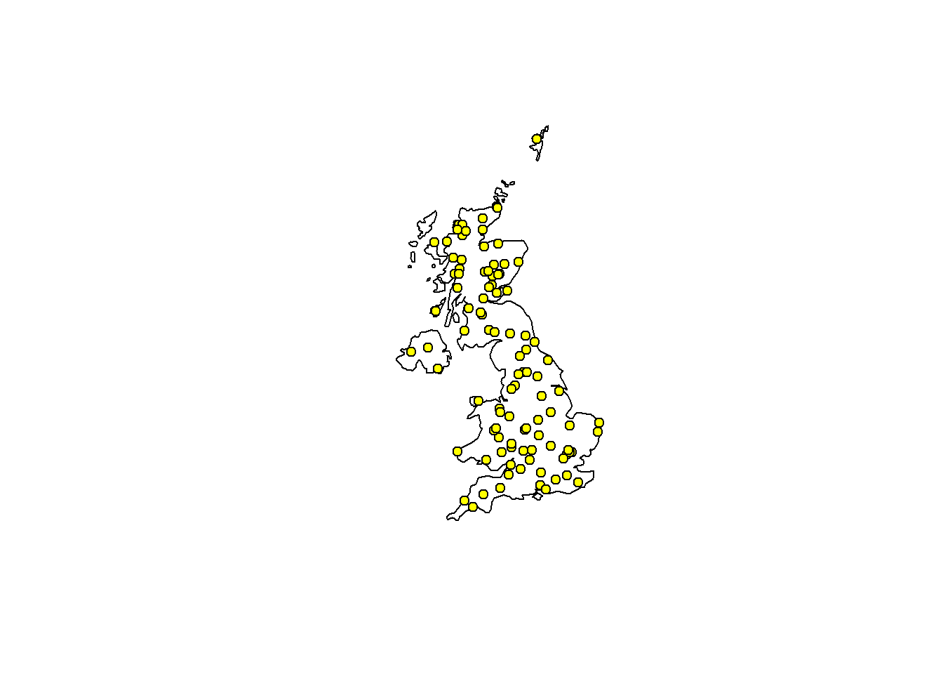
Add points to the map as markers
This code adds the point data to the map as markers and a label for each marker appears on mouse hover.
l2 = l1 %>%
  # Add point data with a label
  addMarkers(
    data = uk_pts,
     # Label appears on mouse hover
     label = paste("Label", seq(1:100)),
     # Options to customise the label text and size
     labelOptions = labelOptions(
       textsize = "14px", # text size
       style = list(
        "font-weight" = "bold", # bold text
        padding = "5px" # padding around text
        )
       )
    )

# widgetframe::frameWidget() function only required to render Leaflet map in RMarkdown
frameWidget(l2, width = "100%", height = "500")
Add tree icons instead of markers to represent the points
# Link to icon
tree_icon = "https://cdn-icons-png.flaticon.com/512/490/490091.png"

l2 = l1 %>%
  # Add point data with a label
  addMarkers(
    data = uk_pts,
    group = "Tree icons",
    # Label appears on mouse hover
    label = paste("Label", seq(1:100)),
    # Options to customise the label text and size
    labelOptions = labelOptions(
      textsize = "14px", # text size
      style = list(
        "font-weight" = "bold", # bold text
        padding = "5px" # padding around text
      )
    ),
    # Change markers to custom icons
    icon = list(
      iconUrl = tree_icon,
      iconSize = c(20, 20)
      )
    )

# widgetframe::frameWidget() function only required to render Leaflet map in RMarkdown
frameWidget(l2, width = "100%", height = "500")3. Add polygon data
Create a polygon using a bounding box of four coordinates
# Boundary box
poly_df = data.frame(lon = c(-1.5,-0.9), lat = c(52.0,52.2))

# Convert to a polygon sf object
poly1 = st_as_sf(poly_df, coords = c("lon","lat"), crs = 4326) %>%
  st_bbox %>%
  st_as_sfc %>%
  st_as_sf
# plot(poly1)
Add polygon to the map
This code creates a blue polygon, the border of which is highlighted white on mouse hover and a popup label appears on mouse click.
l3 = l2 %>%
  # Add polygon to map
  addPolygons(
    data = poly1,
    group = "Polygon 1",
    # stroke parameters
    weight = 3, color = "blue",
    # fill parameters
    fillColor = "blue", fillOpacity = 0.1,
    # Popup label
    popup = "Polygon 1",
    # Options to customise polygon highlighting
    highlightOptions = highlightOptions(
      # Highlight stroke parameters
      weight = 3, color = "white",
      # Highlight fill parameters
      fillColor = "blue", fillOpacity = 0.1
      )
    )

# widgetframe::frameWidget() function only required to render Leaflet map in RMarkdown
frameWidget(l3, width = "100%", height = "500")4. Add popup graphs and images
Sample two additional random points within the UK boundary outline
# Sample two random points and visualise on UK outline
set.seed(1234)
uk_pts2 = st_sample(uk_outline, size = 2)
plot(uk_outline)
plot(uk_pts, pch = 21, col = "black", bg = "yellow", add = TRUE)
plot(uk_pts2, pch = 21, col = "black", bg = "red", add = TRUE)
Prepare graph and image examples to popup on mouse click
# Example graph to show
graph1 = levelplot(t(volcano), col.regions = heat.colors(100), xlab = "", ylab = "")

# Example image to show (GIFs can also be used)
img1 = "https://www.r-project.org/logo/Rlogo.png"
# img1 = "https://upload.wikimedia.org/wikipedia/commons/d/d6/MeanMonthlyP.gif"
Add popup graph and image to the map
This code uses the addPopupGraphs() and addPopupImages() functions from the leafpop package. addPopupGraphs() expects a list of lattice or ggplot2 objects, while addPopupImages expects a vector of file paths or web-URLs to image files. When using more than one graph or image, the number should be the same as the number of points for the popups to render correctly. You may also need to check that the order of the graphs or images matches that of the order of the points so that the correct popup appears on the correct point.
l4 = l3 %>%
  # Add red circle point with a popup graph on mouse click
  addCircles(
    data = uk_pts2[1],
    # group argument essential for linking to popup graph
    group = "Circle point 1",
    # circle size
    radius = 10000,
    # circle stroke parameters
    weight = 1, color = "black",
    # circle fill parameterse
    fillColor = "red", fillOpacity = 0.8,
    # highlight options
    highlightOptions = highlightOptions(
      weight = 1, color = "white", fillOpacity = 0.8
      )
    ) %>%
  # Add popup graph
  addPopupGraphs(
    graph = list(graph1), width = 200, height = 200,
    group = "Circle point 1"
    )%>%
  # Add red circle point with a popup image on mouse click
  addCircles(
    data = uk_pts2[2],
    # group argument essential for linking to popup image
    group = "Circle point 2",
    # circle size
    radius = 10000,
    # circle stroke parameters
    weight = 1, color = "black",
    # circle fill parameterse
    fillColor = "red", fillOpacity = 0.8,
    # highlight options
    highlightOptions = highlightOptions(
      weight = 1, color = "white", fillOpacity = 0.8
      )
    ) %>%
  # Add popup image
  addPopupImages(
    image = img1, width = 100, height = 100,
    group = "Circle point 2"
    )

# widgetframe::frameWidget() function only required to render Leaflet map in RMarkdown
frameWidget(l4, width = "100%", height = "500")5. Add extra customisation and widgets
This code enables the following:
- Button to reset the map view to its default setting
- Minimap display which can be toggled on or off
- Measurement widget to compute distances and areas
- Scale bar
- Layers control switch to toggle layers on or off
- Define the zoom levels for which layers are displayed
l5 = l4 %>%
  # Reset map to default setting
  leaflet.extras::addResetMapButton() %>%
  # Add an inset minimap
  addMiniMap(
    position = "topright",
    tiles = providers$Esri.WorldStreetMap,
    toggleDisplay = TRUE,
    minimized = FALSE
    ) %>%
  # Add measurement tool
  addMeasure(
    position = "topleft",
    primaryLengthUnit = "meters",
    secondaryLengthUnit = "kilometers",
    primaryAreaUnit = "sqmeters"
    ) %>%
  # Add scale bar
  addScaleBar(
    position = "bottomright",
    options = scaleBarOptions(imperial = FALSE)
    ) %>%
  # Add a User-Interface (UI) control to switch layers
  addLayersControl(
    position = "topright",
    baseGroups = c("Open Street Map","ESRI World Imagery","ESRI Ocean Basemap"),
    # Add an option in layer control to toggle layers
    overlayGroups = c("Polygon 1","Circle point 1","Circle point 2","Tree icons"),
    # Choose to permanently display or collapse layers control switch
    options = layersControlOptions(collapsed = TRUE)
    ) %>%
  # Only show tree icons at a defined zoom level
  groupOptions("Tree icons", zoomLevels = 8:20)
6. Final map
7. Further resources and R session info
Leaflet for R: vignette
R package: leaflet.extras
R package: leaflet.extras2
R package: leafpop
R package: leafem
R package: leafgl
sessionInfo()
## R version 4.1.1 (2021-08-10)
## Platform: x86_64-w64-mingw32/x64 (64-bit)
## Running under: Windows 10 x64 (build 19043)
##
## Matrix products: default
##
## locale:
## [1] LC_COLLATE=English_United Kingdom.1252
## [2] LC_CTYPE=English_United Kingdom.1252
## [3] LC_MONETARY=English_United Kingdom.1252
## [4] LC_NUMERIC=C
## [5] LC_TIME=English_United Kingdom.1252
##
## attached base packages:
## [1] stats     graphics  grDevices utils     datasets  methods   base
##
## other attached packages:
##  [1] widgetframe_0.3.1    htmlwidgets_1.5.4    lattice_0.20-44
##  [4] rnaturalearth_0.1.0  forcats_0.5.1        stringr_1.4.0
##  [7] dplyr_1.0.7          purrr_0.3.4          readr_2.1.1
## [10] tidyr_1.1.4          tibble_3.1.5         ggplot2_3.3.5
## [13] tidyverse_1.3.1      sf_1.0-5             htmltools_0.5.2
## [16] leaflet.extras_1.0.0 leafpop_0.1.0        leaflet_2.0.4.1
##
## loaded via a namespace (and not attached):
##  [1] fs_1.5.2                lubridate_1.8.0         httr_1.4.2
##  [4] tools_4.1.1             backports_1.4.1         bslib_0.3.1
##  [7] utf8_1.2.2              R6_2.5.1                KernSmooth_2.23-20
## [10] rgeos_0.5-9             DBI_1.1.2               colorspace_2.0-2
## [13] withr_2.4.3             sp_1.4-5                tidyselect_1.1.1
## [16] rnaturalearthdata_0.1.0 compiler_4.1.1          cli_3.1.0
## [19] rvest_1.0.2             xml2_1.3.3              bookdown_0.24
## [22] sass_0.4.0              scales_1.1.1            classInt_0.4-3
## [25] proxy_0.4-26            systemfonts_1.0.3       digest_0.6.28
## [28] rmarkdown_2.11          svglite_2.0.0           base64enc_0.1-3
## [31] pkgconfig_2.0.3         highr_0.9               dbplyr_2.1.1
## [34] fastmap_1.1.0           rlang_0.4.12            readxl_1.3.1
## [37] rstudioapi_0.13         jquerylib_0.1.4         generics_0.1.1
## [40] jsonlite_1.7.2          crosstalk_1.2.0         magrittr_2.0.1
## [43] s2_1.0.7                Rcpp_1.0.7              munsell_0.5.0
## [46] fansi_0.5.0             lifecycle_1.0.1         stringi_1.7.6
## [49] yaml_2.2.1              grid_4.1.1              crayon_1.4.2
## [52] haven_2.4.3             hms_1.1.1               knitr_1.37
## [55] pillar_1.6.4            uuid_1.0-3              markdown_1.1
## [58] wk_0.5.0                reprex_2.0.1            glue_1.4.2
## [61] evaluate_0.14           blogdown_1.6            leaflet.providers_1.9.0
## [64] modelr_0.1.8            vctrs_0.3.8             tzdb_0.2.0
## [67] cellranger_1.1.0        gtable_0.3.0            assertthat_0.2.1
## [70] xfun_0.27               broom_0.7.10            e1071_1.7-9
## [73] class_7.3-19            units_0.7-2             ellipsis_0.3.2
## [76] brew_1.0-6