Extracting marine data from Bio-ORACLE
Contents
- Explore Bio-ORACLE data sets
- Download and import Bio-ORACLE rasters
- Plot rasters
- Extract data from rasters
- Download pdf and R session info
1. Explore Bio-ORACLE data sets
Bio-ORACLE is a website that allow users to download biotic, geophysical and environmental data for surface and benthic marine realms in raster format. All data layers are available globally at the same spatial resolution of 5 arcmin (approximately 9.2 km at the equator). At the time of writing, Bio-ORACLE also allows you to download future layers for four variables: sea temperature, salinity, current velocity and ice thickness. A list of all available data sets for surface and benthic layers can be found here.
Example applications of Bio-ORACLE marine layers
- Species distribution modelling / Ecological niche modelling
- Seascape genomics
- Genotype-environment associations
- Redundancy analysis
Install and load R packages
library(tidyverse)
library(sdmpredictors)
library(raster)
library(sp)
library(dismo)
Export a csv file containing marine variables of interest
The code below uses the tidyverse packages and regular expressions to extract information for the following variables: sea temperature, salinity, bathymetry, current velocity, dissolved oxygen, primary production, phosphate concentration, pH and silicate concentration. The exported files contain useful information such as the layer codes and descriptions, the units of measurement, and the resolution.
# List marine data sets
datasets = list_datasets(terrestrial = FALSE, marine = TRUE)

# Variables of interest
variables = c("temp","salinity","bathy","curvel","ox","pp","ph","silicate")

# Extract present-day data sets
present = list_layers(datasets) %>%
  # select certain columns
  dplyr::select(dataset_code, layer_code, name, units, description, contains("cellsize"), version) %>%
  # keep variables of interest using a regular expression
  dplyr::filter(grepl(paste(variables, collapse = "|"), layer_code))
# Export present-day data sets to csv file
write_csv(present, path = "bio-oracle-present-datasets.csv")# Future Representative Concentration Pathway (RCP) scenarios of interest
rcp = c("RCP26","RCP45","RCP60","RCP85")
# Extract future data sets
future = list_layers_future(datasets) %>%
# keep RCP scenarios of interest
dplyr::filter(grepl(paste(rcp, collapse = "|"), scenario)) %>%
# keep data for 2050 and 2100
dplyr::filter(year == 2050 | year == 2100) %>%
# keep variables of interest using a regular expression
dplyr::filter(grepl(paste(variables, collapse = "|"), layer_code))# Export future data sets to csv file
write_csv(future, path = "bio-oracle-future-datasets.csv")For the remainder of this post, we will focus on bathymetry and sea temperature but all of the code should be directly applicable to any of the other raster layers.
Check collinearity between sea temperature layers
Variables that are correlated with each other can affect the performance of models downstream. Therefore, if two variables are deemed to be correlated then usually only one of these is used in the analysis. In the example below, we specify the layer codes of our variables of interest and then assess their correlation.
# Create vectors of sea temperature layers
temp.bottom = c("BO2_tempmax_bdmean","BO2_tempmean_bdmean","BO2_tempmin_bdmean","BO2_temprange_bdmean")
temp.surface = c("BO2_tempmax_ss","BO2_tempmean_ss","BO2_tempmin_ss","BO2_temprange_ss")
temp.bottom.surface = c(temp.bottom, temp.surface)

# Check correlation between sea temperature layers
layers_correlation(temp.bottom.surface) %>% plot_correlation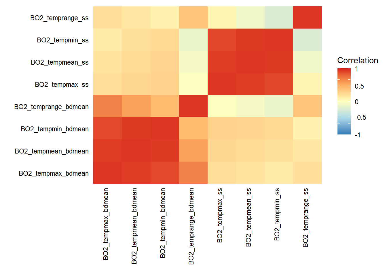
# Re-examine layers that are not correlated (-0.6 > x < 0.6)
temp.present = c("BO2_tempmean_bdmean","BO2_temprange_bdmean","BO2_tempmean_ss","BO2_temprange_ss")
layers_correlation(temp.present) %>% round(digits = 2)
##                      BO2_tempmean_bdmean BO2_temprange_bdmean BO2_tempmean_ss
## BO2_tempmean_bdmean                 1.00                 0.59            0.24
## BO2_temprange_bdmean                0.59                 1.00           -0.08
## BO2_tempmean_ss                     0.24                -0.08            1.00
## BO2_temprange_ss                    0.15                 0.38           -0.11
##                      BO2_temprange_ss
## BO2_tempmean_bdmean              0.15
## BO2_temprange_bdmean             0.38
## BO2_tempmean_ss                 -0.11
## BO2_temprange_ss                 1.00
layers_correlation(temp.present) %>% plot_correlation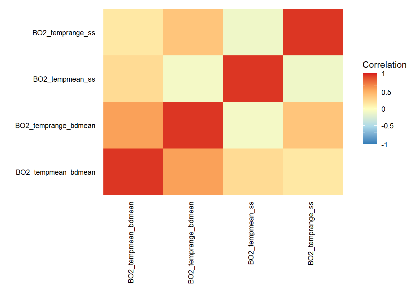
Note that the version of the layers_correlation() function used in this post does not accept version 2.1 of the layers (e.g. BO21_tempmean_bdmean) so version 2.0 was used to illustrate the code above.
2. Download and import Bio-ORACLE rasters
Create vectors containing layer codes to download (version 2.1). Then combine these two vectors into one vector.
# Create vectors containing layer codes to download (version 2.1)
temp.present = gsub("BO2", "BO21", temp.present)
temp.future = c("BO21_RCP26_2050_tempmean_bdmean","BO21_RCP45_2050_tempmean_bdmean","BO21_RCP60_2050_tempmean_bdmean","BO21_RCP85_2050_tempmean_bdmean",
                "BO21_RCP26_2100_tempmean_bdmean","BO21_RCP45_2100_tempmean_bdmean","BO21_RCP60_2100_tempmean_bdmean","BO21_RCP85_2100_tempmean_bdmean",
                "BO21_RCP26_2050_temprange_bdmean","BO21_RCP45_2050_temprange_bdmean","BO21_RCP60_2050_temprange_bdmean","BO21_RCP85_2050_temprange_bdmean",
                "BO21_RCP26_2100_temprange_bdmean","BO21_RCP45_2100_temprange_bdmean","BO21_RCP60_2100_temprange_bdmean","BO21_RCP85_2100_temprange_bdmean",
                "BO21_RCP26_2050_tempmean_ss","BO21_RCP45_2050_tempmean_ss","BO21_RCP60_2050_tempmean_ss","BO21_RCP85_2050_tempmean_ss",
                "BO21_RCP26_2100_tempmean_ss","BO21_RCP45_2100_tempmean_ss","BO21_RCP60_2100_tempmean_ss","BO21_RCP85_2100_tempmean_ss",
                "BO21_RCP26_2050_temprange_ss","BO21_RCP45_2050_temprange_ss","BO21_RCP60_2050_temprange_ss","BO21_RCP85_2050_temprange_ss",
                "BO21_RCP26_2100_temprange_ss","BO21_RCP45_2100_temprange_ss","BO21_RCP60_2100_temprange_ss","BO21_RCP85_2100_temprange_ss"
                )

# Combine present-day and future vectors
temp = c(temp.present, temp.future)
Download raster layers to the sdmpredictors/Meta folder and import the rasters into R. If the rasters have already been downloaded then R will only import the data.
# Download rasters to sdmpredictors/Meta folder and import into R
options(sdmpredictors_datadir = "C:/R-4.0.2/library/sdmpredictors/Meta/")
bathy.raster = load_layers("MS_bathy_5m")
names(bathy.raster) = "MS_bathy_5m"
temp.rasters = load_layers(temp)
## Warning in load_layers(temp): Layers from different eras (current, future,
## paleo) are being loaded together3. Plot rasters
Define a boundary and crop rasters to this extent.
# Define a boundary
boundary = extent(c(xmin = -11.5, xmax = 2.5, ymin = 49.6, ymax = 57))

# Crop rasters to boundary extent
bathy.raster = crop(bathy.raster, boundary)
temp.rasters = crop(temp.rasters, boundary)
Plot rasters using raster::plot() function.
# Define colour scheme
cols = colorRampPalette(c("#5E85B8","#EDF0C0","#C13127"))

# Plot mean bottom mean temperature
raster::subset(temp.rasters, grep("tempmean_bdmean", names(temp.rasters), value = TRUE)) %>%
  plot(col = cols(100), zlim = c(0,17), axes = FALSE, box = FALSE)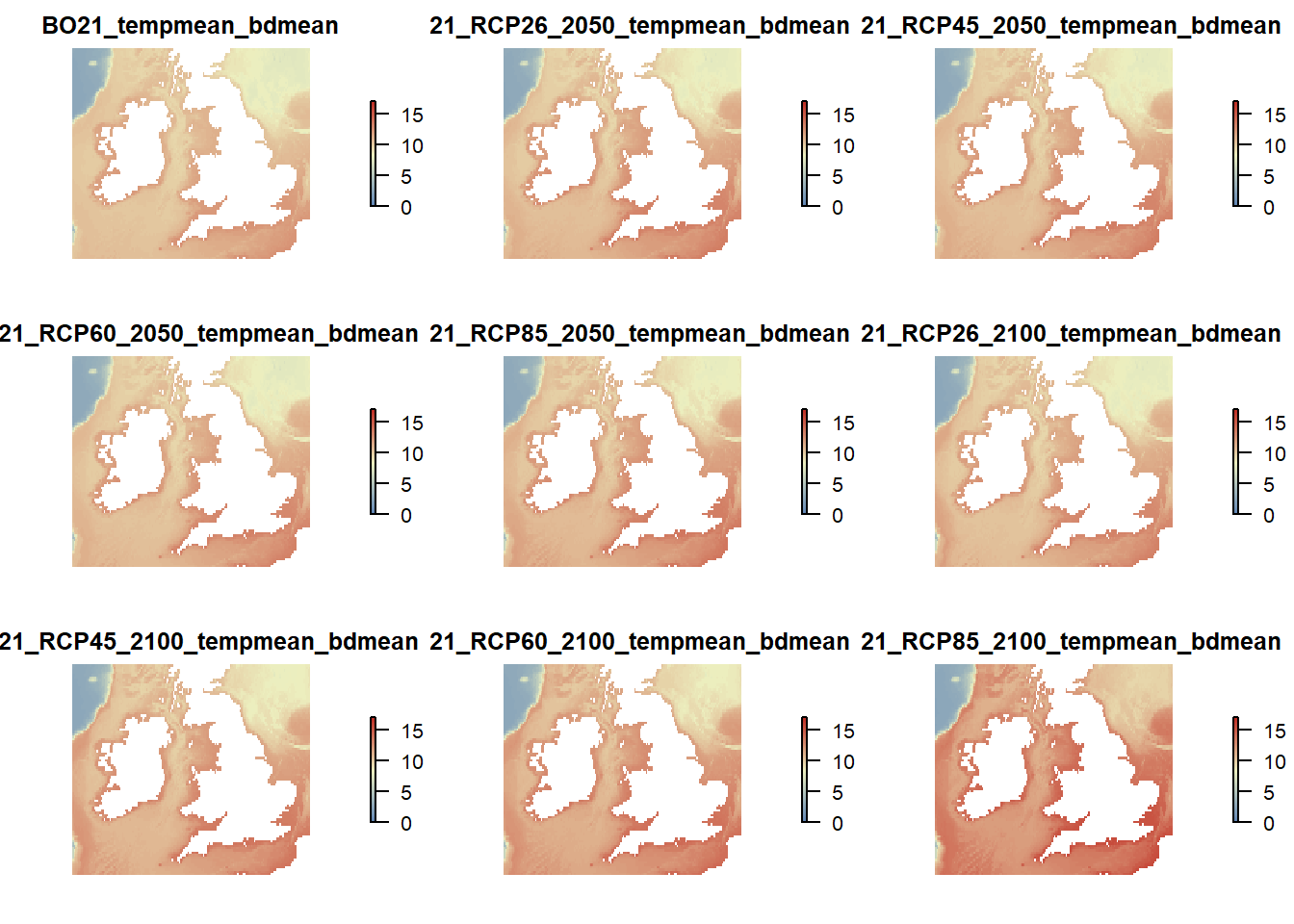
# Plot sea surface mean temperature
raster::subset(temp.rasters, grep("tempmean_ss", names(temp.rasters), value = TRUE)) %>%
  plot(col = cols(100), zlim = c(9,17), axes = FALSE, box = FALSE)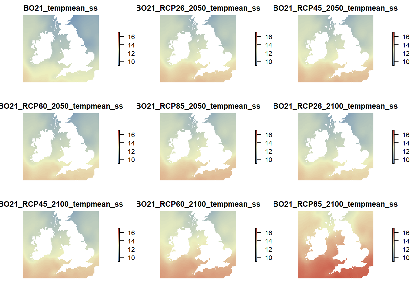
# Plot mean bottom temperature range
raster::subset(temp.rasters, grep("temprange_bdmean", names(temp.rasters), value = TRUE)) %>%
  plot(col = cols(100), zlim = c(0,16), axes = FALSE, box = FALSE)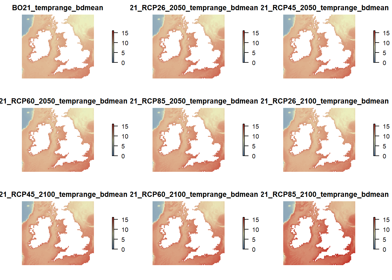
Plot rasters using sp::spplot() function.
# Plot bathymetry up to 200 m depth
sp::spplot(bathy.raster, zlim = c(-200, 0), main = names(bathy.raster),
           scales = list(draw=TRUE), col.regions = topo.colors(100))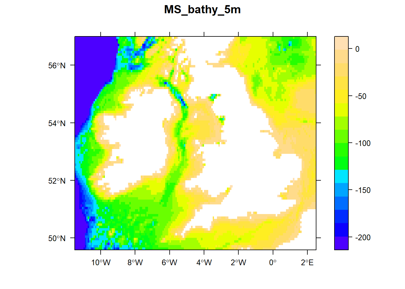
4. Extract data from rasters
Prepare point data
Create or import a file containing longitude and latitude points. In this example, we will create 100 random points directly from a raster layer.
set.seed(123)
random.pts = randomPoints(bathy.raster, n = 100) %>% as_tibble()
Convert tibble to a SpatialPoints object and set coordinate reference system (CRS).
random.pts = SpatialPoints(random.pts, proj4string = CRS("+proj=longlat +datum=WGS84"))
random.pts
## class       : SpatialPoints
## features    : 100
## extent      : -11.45833, 2.458333, 49.70833, 56.95833  (xmin, xmax, ymin, ymax)
## crs         : +proj=longlat +datum=WGS84 +no_defs
Check points CRS matches raster CRS.
projection(random.pts) == projection(bathy.raster)
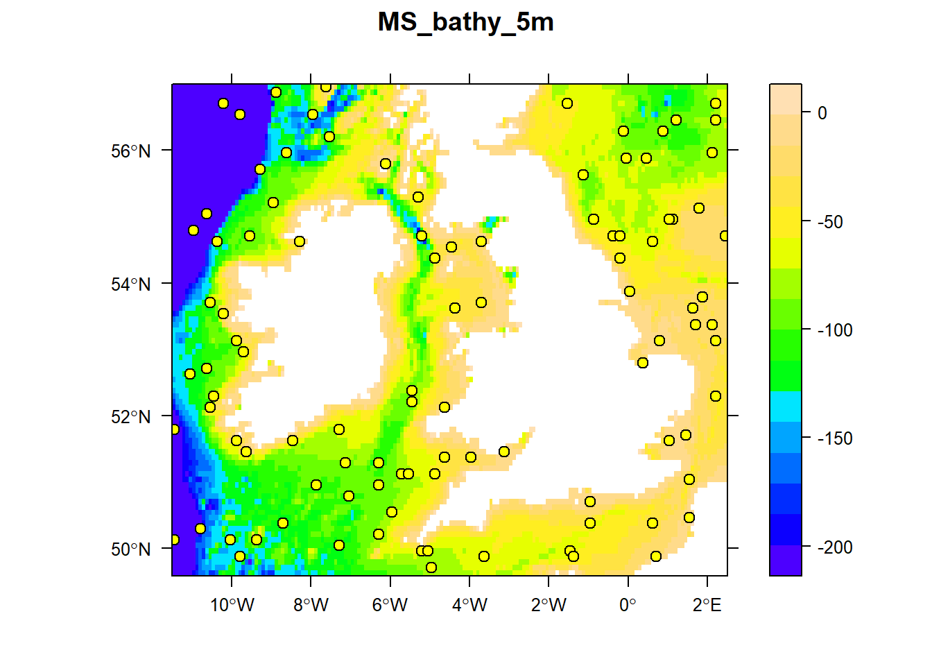
## [1] TRUEPlot points over bathymetry raster.
# raster::plot(bathy.raster, axes = TRUE, box = TRUE, main = names(bathy.raster))
# points(random.pts$x, random.pts$y, pch = 21, cex = 1, bg = "yellow", col = "black")
sp::spplot(bathy.raster, zlim = c(-200, 0), main = names(bathy.raster),
           scales = list(draw=TRUE), col.regions = topo.colors(100),
           sp.layout = c("sp.points", random.pts, pch = 21, cex = 1, fill = "yellow", col = "black")
           )
Create a tibble or data.frame to store Bio-ORACLE marine data for each point.
marine.data = tibble(ID = 1:nrow(random.pts@coords),
                     Lon = random.pts$x,
                     Lat = random.pts$y
                     )
marine.data
## # A tibble: 100 x 3
##       ID     Lon   Lat
##    <int>   <dbl> <dbl>
##  1     1   2.21   52.3
##  2     2  -0.125  56.3
##  3     3  -9.88   53.1
##  4     4  -3.62   49.9
##  5     5 -10.6    55.0
##  6     6  -3.71   53.7
##  7     7 -10.2    53.5
##  8     8  -3.96   51.4
##  9     9  -7.88   51.0
## 10    10 -10.8    50.3
## # ... with 90 more rows
Extract data for each point
Combine all rasters into one raster stack.
rasters = raster::stack(bathy.raster, temp.rasters)
nlayers(rasters)
## [1] 37
Extract data from each raster layer for each point and store in a list.
store_data = list()
for (i in 1:nlayers(rasters)){
  store_data[[i]] = raster::extract(rasters[[i]], random.pts)
}
Add the extracted data as new columns to marine.data.
# Name variables in the list and then combine data
names(store_data) = names(rasters)
marine.data = bind_cols(marine.data, as_tibble(store_data))
marine.data
## # A tibble: 100 x 40
##       ID     Lon   Lat MS_bathy_5m BO21_tempmean_bdmean BO21_temprange_bdmean
##    <int>   <dbl> <dbl>       <dbl>                <dbl>                 <dbl>
##  1     1   2.21   52.3         -37                10.2                  10.2
##  2     2  -0.125  56.3         -89                 7.92                  7.92
##  3     3  -9.88   53.1         -61                10.2                  10.2
##  4     4  -3.62   49.9         -64                11.3                  11.3
##  5     5 -10.6    55.0       -2101                 3.32                  3.32
##  6     6  -3.71   53.7         -32                11.0                  11.0
##  7     7 -10.2    53.5         -21                11.4                  11.4
##  8     8  -3.96   51.4         -28                11.8                  11.8
##  9     9  -7.88   51.0        -103                10.4                  10.4
## 10    10 -10.8    50.3        -187                10.8                  10.8
## # ... with 90 more rows, and 34 more variables: BO21_tempmean_ss <dbl>,
## #   BO21_temprange_ss <dbl>, BO21_RCP26_2050_tempmean_bdmean <dbl>,
## #   BO21_RCP45_2050_tempmean_bdmean <dbl>,
## #   BO21_RCP60_2050_tempmean_bdmean <dbl>,
## #   BO21_RCP85_2050_tempmean_bdmean <dbl>,
## #   BO21_RCP26_2100_tempmean_bdmean <dbl>,
## #   BO21_RCP45_2100_tempmean_bdmean <dbl>, ...
Check for NA values and drop rows if required.
# Check each column for NA values
na.check = map_int(marine.data, ~sum(is.na(.)))
summary(na.check > 0)
##    Mode   FALSE
## logical      40
# Remove NA records
# marine.data = marine.data %>% drop_naRound sea temperature values to three decimal places.
marine.data[-(1:4)] = apply(marine.data[-(1:4)], MARGIN = 2, FUN = round, digits = 3)Visualise the spread of present-day sea temperature values for our points data set.
# Prepare a custom theme for ggplot
theme1 = theme(
  panel.grid.major.x = element_blank(),
  panel.grid.minor.y = element_blank(),
  axis.text = element_text(size = 9, face = "bold"),
  axis.title = element_text(size = 12, face = "bold")
  )

# Violin plot and raw data
marine.data %>%
  # select only columns 5-8 (present-day sea temperature variables)
  dplyr::select(5:8) %>%
  # transform data to long format for plotting
  pivot_longer(names_to = "Variable", values_to = "Values", cols = everything()) %>%
  # plot data
  ggplot(data = .)+
    geom_violin(aes(x = Variable, y = Values, fill = Variable), show.legend = FALSE)+
    geom_jitter(aes(x = Variable, y = Values), show.legend = FALSE, alpha = 0.30)+
    scale_y_continuous(expand = c(0,0), limits = c(0,16), breaks = c(seq(0,16,2)))+
    scale_fill_manual(values = heat.colors(4))+
    xlab("Raster layer")+
    ylab(expression(bold("Temperature ("^o*"C)")))+
    theme1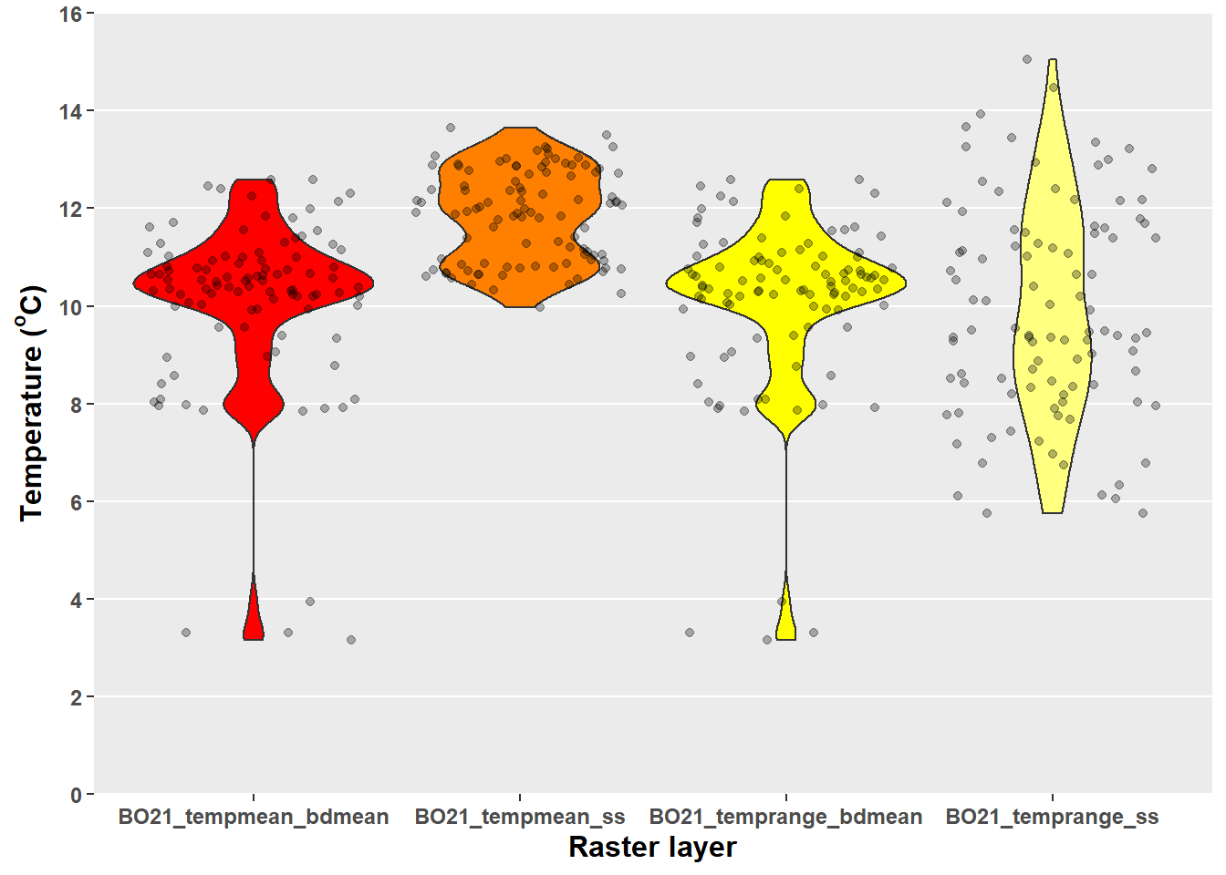
Calculate the deepest and shallowest point.
marine.data %>%
  summarise(deepest = min(MS_bathy_5m), shallowest = max(MS_bathy_5m))
## # A tibble: 1 x 2
##   deepest shallowest
##     <dbl>      <dbl>
## 1   -2101         -2
Export data to a csv file.
write_csv(marine.data, path = "marine_data.csv")5. Download pdf and R session info
Download a PDF of this post here
sessionInfo()
## R version 4.1.1 (2021-08-10)
## Platform: x86_64-w64-mingw32/x64 (64-bit)
## Running under: Windows 10 x64 (build 19043)
##
## Matrix products: default
##
## locale:
## [1] LC_COLLATE=English_United Kingdom.1252
## [2] LC_CTYPE=English_United Kingdom.1252
## [3] LC_MONETARY=English_United Kingdom.1252
## [4] LC_NUMERIC=C
## [5] LC_TIME=English_United Kingdom.1252
##
## attached base packages:
## [1] stats     graphics  grDevices utils     datasets  methods   base
##
## other attached packages:
##  [1] dismo_1.3-5          raster_3.5-2         sp_1.4-5
##  [4] sdmpredictors_0.2.11 forcats_0.5.1        stringr_1.4.0
##  [7] dplyr_1.0.7          purrr_0.3.4          readr_2.1.1
## [10] tidyr_1.1.4          tibble_3.1.5         ggplot2_3.3.5
## [13] tidyverse_1.3.1
##
## loaded via a namespace (and not attached):
##  [1] Rcpp_1.0.7       lubridate_1.8.0  lattice_0.20-44  assertthat_0.2.1
##  [5] digest_0.6.28    utf8_1.2.2       plyr_1.8.6       R6_2.5.1
##  [9] cellranger_1.1.0 backports_1.4.1  reprex_2.0.1     evaluate_0.14
## [13] highr_0.9        httr_1.4.2       blogdown_1.6     pillar_1.6.4
## [17] rlang_0.4.12     readxl_1.3.1     rstudioapi_0.13  jquerylib_0.1.4
## [21] rmarkdown_2.11   rgdal_1.5-28     munsell_0.5.0    broom_0.7.10
## [25] compiler_4.1.1   modelr_0.1.8     xfun_0.27        pkgconfig_2.0.3
## [29] htmltools_0.5.2  tidyselect_1.1.1 bookdown_0.24    codetools_0.2-18
## [33] fansi_0.5.0      crayon_1.4.2     tzdb_0.2.0       dbplyr_2.1.1
## [37] withr_2.4.3      grid_4.1.1       jsonlite_1.7.2   gtable_0.3.0
## [41] lifecycle_1.0.1  DBI_1.1.2        magrittr_2.0.1   scales_1.1.1
## [45] cli_3.1.0        stringi_1.7.6    farver_2.1.0     reshape2_1.4.4
## [49] fs_1.5.2         xml2_1.3.3       bslib_0.3.1      ellipsis_0.3.2
## [53] generics_0.1.1   vctrs_0.3.8      tools_4.1.1      glue_1.4.2
## [57] hms_1.1.1        fastmap_1.1.0    yaml_2.2.1       terra_1.4-11
## [61] colorspace_2.0-2 rvest_1.0.2      knitr_1.37       haven_2.4.3
## [65] sass_0.4.0