Getting started with population genetics using R
Contents
1. Why bother with R?
There are so many programs and software out there for analysing population genetic data and generating summary statistics. At first I was quite overwhelmed and unsure which path to take. Then I started learning and using R and I’ve not looked back since. Aside from the fact that R was the first programming language I learnt, there are several reasons why I like to use R for popgen analysis:
- A wealth of online help resources and tutorials
- Analyses easily replicated on new data sets
- Many options for creating publication quality figures and visualisations
- Code can be uploaded to online repositories for other people to reproduce your analysis
- Cross platform compatibility
- Free!
Nowadays, popgen R has dozens of packages that often allow you to do similar things but different packages can have their own formatting requirements and R objects. I recommend choosing one type of R object to conduct all your analyses with because converting between R objects can be difficult and frustrating (I work with genind objects from the adegenet package).
In this post, I cover some ‘bread-and-butter’ analyses for typical popgen data sets and highlight some of the R packages and functions I use to analyse such data using example data sets from published studies.
Assumptions
This post assumes that you have installed R and RStudio and that you have some skills in R coding and functionality. To follow along, I recommend that you download the example data sets to a directory of your choice, create a new R script in the same directory and then set your working directory to the location of these files. To set your working directory in RStudio, for example, click Session > Set Working Directory > To Source File Location.
Download example data sets
1. European lobster SNP genotypes in data.frame format
2. Pink sea fan microsatellite genotypes in genepop format
References
Jenkins TL, Ellis CD, Triantafyllidis A, Stevens JR (2019). Single nucleotide polymorphisms reveal a genetic cline across the north‐east Atlantic and enable powerful population assignment in the European lobster. Evolutionary Applications 12, 1881–1899.
Holland LP, Jenkins TL, Stevens JR (2017). Contrasting patterns of population structure and gene flow facilitate exploration of connectivity in two widely distributed temperate octocorals. Heredity 119, 35–48.
2. Import genetic data
Install and load R packages
library(adegenet)
library(poppr)
library(dplyr)
library(hierfstat)
library(reshape2)
library(ggplot2)
library(RColorBrewer)
library(scales)
Import lobster SNP genotypes
Import csv file containing SNP (single nucleotide polymorphism) genotypes.
lobster = read.csv("Lobster_SNP_Genotypes.csv")
str(lobster)
## 'data.frame':    125280 obs. of  4 variables:
##  $ Site    : chr  "Ale" "Ale" "Ale" "Ale" ...
##  $ ID      : chr  "Ale04" "Ale04" "Ale04" "Ale04" ...
##  $ Locus   : int  3441 4173 6157 7502 7892 8953 9441 11071 11183 11291 ...
##  $ Genotype: chr  "GG" NA NA NA ...
Convert data.frame from long to wide format. The wide format contains one row for each individual and one column for each locus as well as a column for the ID and site labels.
lobster_wide = reshape(lobster, idvar = c("ID","Site"), timevar = "Locus", direction = "wide", sep = "")
## Warning in reshapeWide(data, idvar = idvar, timevar = timevar, varying =
## varying, : multiple rows match for Locus=3441: first taken

# Remove "Genotype" from column names
colnames(lobster_wide) = gsub("Genotype", "", colnames(lobster_wide))
Subset genotypes and only keep SNP loci used in Jenkins et al. 2019.
# Subset genotypes
snpgeno = lobster_wide[ , 3:ncol(lobster_wide)]

# Keep only SNP loci used in Jenkins et al. 2019
snps_to_remove = c("25580","32362","41521","53889","65376","8953","21197","15531","22740","28357","33066","51507","53052","53263","21880","22323","22365")
snpgeno = snpgeno[ , !colnames(snpgeno) %in% snps_to_remove]
Create vectors of individual and site labels.
ind = as.character(lobster_wide$ID) # individual ID
site = as.character(lobster_wide$Site) # site ID
Convert data.frame to genind object. Check that the genotypes for the first five individuals and loci are as expected.
lobster_gen = df2genind(snpgeno, ploidy = 2, ind.names = ind, pop = site, sep = "")
lobster_gen$tab[1:5, 1:10]
##       3441.G 3441.A 4173.C 4173.T 6157.G 6157.C 7502.T 7502.C 7892.T 7892.A
## Ale04      2      0     NA     NA     NA     NA     NA     NA      2      0
## Ale05      1      1      2      0      1      1      2      0      1      1
## Ale06     NA     NA      2      0      2      0     NA     NA      2      0
## Ale08     NA     NA      0      2      2      0      2      0     NA     NA
## Ale13      2      0     NA     NA      2      0     NA     NA      2      0
Print basic info of the genind object.
lobster_gen
## /// GENIND OBJECT /////////
##
##  // 1,305 individuals; 79 loci; 158 alleles; size: 945.1 Kb
##
##  // Basic content
##    @tab:  1305 x 158 matrix of allele counts
##    @loc.n.all: number of alleles per locus (range: 2-2)
##    @loc.fac: locus factor for the 158 columns of @tab
##    @all.names: list of allele names for each locus
##    @ploidy: ploidy of each individual  (range: 2-2)
##    @type:  codom
##    @call: df2genind(X = snpgeno, sep = "", ind.names = ind, pop = site,
##     ploidy = 2)
##
##  // Optional content
##    @pop: population of each individual (group size range: 7-41)

popNames(lobster_gen)
##  [1] "Ale"   "Ber"   "Brd"   "Cor"   "Cro"   "Eye"   "Flo"   "Gul"   "Heb"
## [10] "Hel"   "Hoo"   "Idr16" "Idr17" "Iom"   "Ios"   "Jer"   "Kav"   "Kil"
## [19] "Laz"   "Loo"   "Lyn"   "Lys"   "Mul"   "Oos"   "Ork"   "Pad"   "Pem"
## [28] "Sar13" "Sar17" "Sbs"   "She"   "Sin"   "Sky"   "Sul"   "Tar"   "The"
## [37] "Tor"   "Tro"   "Ven"   "Vig"
Import pink sea fan microsatellite genotypes
Import genepop file and convert to genind object. Check that the genotypes at locus Ever002 for three randomly selected individuals are as expected.
seafan_gen = import2genind("Pinkseafan_13MicrosatLoci.gen", ncode = 3, quiet = TRUE)
set.seed(1)
tab(seafan_gen[loc = "Ever002"])[runif(3, 1, nInd(seafan_gen)), ]
##       Ever002.114 Ever002.117 Ever002.109 Ever002.105 Ever002.121
## Far10           2           0           0           0           0
## Han36           2           0           0           0           0
## Moh5            1           1           0           0           0
Print basic info of the genind object.
seafan_gen
## /// GENIND OBJECT /////////
##
##  // 877 individuals; 13 loci; 114 alleles; size: 478.2 Kb
##
##  // Basic content
##    @tab:  877 x 114 matrix of allele counts
##    @loc.n.all: number of alleles per locus (range: 2-18)
##    @loc.fac: locus factor for the 114 columns of @tab
##    @all.names: list of allele names for each locus
##    @ploidy: ploidy of each individual  (range: 2-2)
##    @type:  codom
##    @call: read.genepop(file = file, ncode = 3, quiet = quiet)
##
##  // Optional content
##    @pop: population of each individual (group size range: 22-48)

popNames(seafan_gen)
##  [1] "ArmI_27"   "ArmII_43"  "ArmIII_41" "Bla29"     "Bov40"     "Bre43"
##  [7] "Far44"     "Fla23"     "Han36"     "Lao40"     "Lio22"     "Lun22"
## [13] "Men43"     "Mew44"     "Moh30"     "PorI_42"   "PorII_35"  "Rag43"
## [19] "RosI_40"   "RosII_36"  "Sko39"     "Thu48"     "Vol24"     "Wtn43"
Update the site labels so that the site code rather than the last individual label in the sample is used.
# Use gsub to extract only letters from a vector
popNames(seafan_gen) = gsub("[^a-zA-Z]", "", popNames(seafan_gen))
popNames(seafan_gen)
##  [1] "ArmI"   "ArmII"  "ArmIII" "Bla"    "Bov"    "Bre"    "Far"    "Fla"
##  [9] "Han"    "Lao"    "Lio"    "Lun"    "Men"    "Mew"    "Moh"    "PorI"
## [17] "PorII" "Rag" "RosI" "RosII" "Sko" "Thu" "Vol" "Wtn"3. Filtering
Missing data: loci
Calculate the percentage of complete genotypes per loci in the lobster SNP data set.
locmiss_lobster = propTyped(lobster_gen, by = "loc")
locmiss_lobster[which(locmiss_lobster < 0.80)] # print loci with < 80% complete genotypes
## named numeric(0)

# Barplot
barplot(locmiss_lobster, ylim = c(0,1), ylab = "Complete genotypes (proportion)", xlab = "Locus", las = 2, cex.names = 0.7)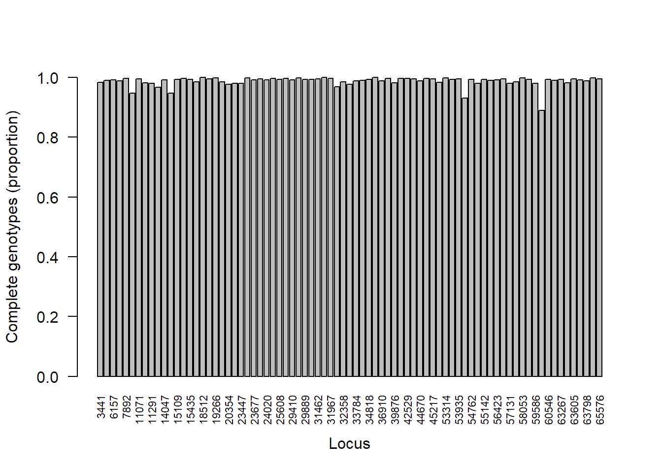
Calculate the percentage of complete genotypes per loci in the pink sea fan microsatellite data set.
locmiss_seafan = propTyped(seafan_gen, by = "loc")
locmiss_seafan[which(locmiss_seafan < 0.80)] # print loci with < 80% complete genotypes
##   Ever012
## 0.6294185

# Barplot
barplot(locmiss_seafan, ylim = c(0,1), ylab = "Complete genotypes (proportion)", xlab = "Locus", las = 2, cex.names = 0.7)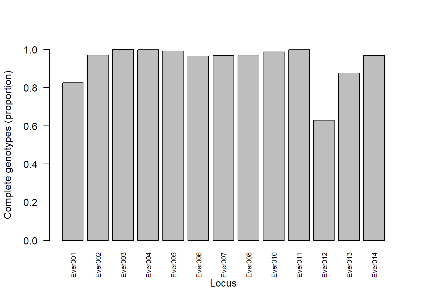
Remove microsatellite loci with > 20% missing data.
seafan_gen = missingno(seafan_gen, type = "loci", cutoff = 0.20)
##
## Found 6873 missing values.
##
## 1 locus contained missing values greater than 20%
##
## Removing 1 locus: , Ever012
Missing data: individuals
Calculate the percentage of complete genotypes per individual in the lobster SNP data set.
indmiss_lobster = propTyped(lobster_gen, by = "ind")
indmiss_lobster[ which(indmiss_lobster < 0.80) ] # print individuals with < 80% complete genotypes
##     Ale04     Ale06     Ale08     Ale13     Ale15     Ale16     Ale19     Sin65
## 0.4936709 0.5063291 0.5443038 0.5696203 0.4556962 0.5316456 0.4430380 0.7848101
##     The24
## 0.5696203
Remove individuals with > 20% missing genotypes.
lobster_gen = missingno(lobster_gen, type = "geno", cutoff = 0.20)
##
## Found 2590 missing values.
##
## 9 genotypes contained missing values greater than 20%
##
## Removing 9 genotypes: Ale04, Ale06, Ale08, Ale13, Ale15, Ale16, Ale19,
## Sin65, The24
Calculate the percentage of complete genotypes per individual in the pink sea fan microsatellite data set.
indmiss_seafan= propTyped(seafan_gen, by = "ind")
indmiss_seafan[ which(indmiss_seafan < 0.80) ] # print individuals with < 80% complete genotypes
##  ArmIII_9 ArmIII_31      Bov1     Bov39     Lao11     Lao13     Lao16     Lao34
##      0.75      0.75      0.75      0.75      0.75      0.75      0.75      0.75
##     Lun19      Moh8     Moh29   PorI_25   PorI_33   PorI_40   PorII_7     Rag14
##      0.75      0.75      0.75      0.75      0.75      0.75      0.75      0.75
##   RosI_33  RosII_36     Vol21
##      0.75      0.75      0.75
Remove individuals with > 20% missing genotypes.
seafan_gen = missingno(seafan_gen, type = "geno", cutoff = 0.20)
##
## Found 5248 missing values.
##
## 19 genotypes contained missing values greater than 20%
##
## Removing 19 genotypes: ArmIII_9, ArmIII_31, Bov1, Bov39, Lao11, Lao13,
## Lao16, Lao34, Lun19, Moh8, Moh29, PorI_25, PorI_33, PorI_40, PorII_7,
## Rag14, RosI_33, RosII_36, Vol21
Check genotypes are unique
Check all individual genotypes are unique. Duplicated genotypes can result from unintentionally sampling the same individual twice or from sampling clones.
# Print the number of multilocus genotypes
mlg(lobster_gen)
## #############################
## # Number of Individuals:  1296
## # Number of MLG:  1271
## #############################
## [1] 1271

mlg(seafan_gen)
## #############################
## # Number of Individuals:  858
## # Number of MLG:  857
## #############################
## [1] 857
Identify duplicated genotypes.
dups_lobster = mlg.id(lobster_gen)
for (i in dups_lobster){ # for each element in the list object
  if (length(dups_lobster[i]) > 1){ # if the length is greater than 1
    print(i) # print individuals that are duplicates
  }
}
## [1] "Laz4" "Tar4"
## [1] "Eye15" "Eye16" "Eye35"
## [1] "Eye01" "Eye17"
## [1] "Laz2" "Tar2"
## [1] "Eye08" "Eye41"
## [1] "Gul101" "Gul86"
## [1] "Eye25" "Eye29"
## [1] "Iom02" "Iom22"
## [1] "Hel07" "Hel09"
## [1] "Eye27" "Eye42"
## [1] "Eye05" "Eye06" "Eye23" "Eye40"
## [1] "Eye22" "Eye38"
## [1] "Eye11" "Eye32"
## [1] "Cro08" "Cro15"
## [1] "Laz1" "Tar1"
## [1] "Eye14" "Eye31"
## [1] "Laz3" "Tar3"
## [1] "Lyn04" "Lyn15" "Lyn34"
## [1] "Eye07" "Eye24"
## [1] "Eye02" "Eye04"
## [1] "Eye20" "Eye36"

dups_seafan = mlg.id(seafan_gen)
for (i in dups_seafan){ # for each element in the list object
  if (length(dups_seafan[i]) > 1){ # if the length is greater than 1
    print(i) # print individuals that are duplicates
  }
}
## [1] "ArmI_15" "ArmII_2"
Remove duplicated genotypes.
# Create a vector of individuals to remove
lob_dups = c("Laz4","Eye15","Eye16","Eye01","Laz2","Eye08","Gul101","Eye25","Iom02","Hel07","Eye27","Eye05","Eye06","Eye23","Eye22","Eye11","Cro08","Tar1","Eye14","Tar3","Lyn04","Lyn15","Eye07","Eye02","Eye20")
psf_dups = c("ArmI_15")
# Create a vector of individual names without the duplicates
lob_Nodups = indNames(lobster_gen)[! indNames(lobster_gen) %in% lob_dups]
psf_Nodups = indNames(seafan_gen)[! indNames(seafan_gen) %in% psf_dups]# Create a new genind object without the duplicates
lobster_gen = lobster_gen[lob_Nodups, ]
seafan_gen = seafan_gen[psf_Nodups, ]# Re-print the number of multilocus genotypes
mlg(lobster_gen)
## #############################
## # Number of Individuals: 1271
## # Number of MLG: 1271
## #############################
## [1] 1271
mlg(seafan_gen)
## #############################
## # Number of Individuals: 857
## # Number of MLG: 857
## #############################
## [1] 857Check loci are still polymorphic after filtering
isPoly(lobster_gen) %>% summary
##    Mode    TRUE
## logical      79

isPoly(seafan_gen) %>% summary
##    Mode   FALSE    TRUE
## logical       1      11
Remove loci that are not polymorphic.
poly_loci = names(which(isPoly(seafan_gen) == TRUE))
seafan_gen = seafan_gen[loc = poly_loci]
isPoly(seafan_gen) %>% summary
##    Mode    TRUE
## logical 114. Summary statistics
Print basic info
lobster_gen
## /// GENIND OBJECT /////////
##
##  // 1,271 individuals; 79 loci; 158 alleles; size: 921.5 Kb
##
##  // Basic content
##    @tab:  1271 x 158 matrix of allele counts
##    @loc.n.all: number of alleles per locus (range: 2-2)
##    @loc.fac: locus factor for the 158 columns of @tab
##    @all.names: list of allele names for each locus
##    @ploidy: ploidy of each individual  (range: 2-2)
##    @type:  codom
##    @call: .local(x = x, i = i, j = j, drop = drop)
##
##  // Optional content
##    @pop: population of each individual (group size range: 5-40)

seafan_gen
## /// GENIND OBJECT /////////
##
##  // 857 individuals; 11 loci; 106 alleles; size: 439.8 Kb
##
##  // Basic content
##    @tab:  857 x 106 matrix of allele counts
##    @loc.n.all: number of alleles per locus (range: 2-18)
##    @loc.fac: locus factor for the 106 columns of @tab
##    @all.names: list of allele names for each locus
##    @ploidy: ploidy of each individual  (range: 2-2)
##    @type:  codom
##    @call: .local(x = x, i = i, j = j, loc = ..1, drop = drop)
##
##  // Optional content
##    @pop: population of each individual (group size range: 21-48)
Print the number of alleles per locus
table(lobster_gen$loc.fac)
##
##  3441  4173  6157  7502  7892  9441 11071 11183 11291 12971 14047 14742 15109
##     2     2     2     2     2     2     2     2     2     2     2     2     2
## 15128 15435 15581 18512 18652 19266 19460 20354 23146 23447 23481 23677 23787
##     2     2     2     2     2     2     2     2     2     2     2     2     2
## 24020 25229 25608 27329 29410 29801 29889 30339 31462 31618 31967 31979 32358
##     2     2     2     2     2     2     2     2     2     2     2     2     2
## 32435 33784 34443 34818 35584 36910 39107 39876 42395 42529 42821 44670 45154
##     2     2     2     2     2     2     2     2     2     2     2     2     2
## 45217 51159 53314 53720 53935 54240 54762 55111 55142 55564 56423 56785 57131
##     2     2     2     2     2     2     2     2     2     2     2     2     2
## 57989 58053 59503 59586 59967 60546 63140 63267 63581 63605 63771 63798 65064
##     2     2     2     2     2     2     2     2     2     2     2     2     2
## 65576
##     2

table(seafan_gen$loc.fac)
##
## Ever001 Ever002 Ever003 Ever004 Ever006 Ever007 Ever008 Ever010 Ever011 Ever013
##      15       5       5      13      18      11       2       9       5      14
## Ever014
##       9
Print the sample size for each site
summary(lobster_gen$pop)
##   Ale   Ber   Brd   Cor   Cro   Eye   Flo   Gul   Heb   Hel   Hoo Idr16 Idr17
##    28    33    36    32    35    26    36    35    36    35    36    32    29
##   Iom   Ios   Jer   Kav   Kil   Laz   Loo   Lyn   Lys   Mul   Oos   Ork   Pad
##    35    36    36    36    35     5    36    34    36    36    40    36    36
##   Pem Sar13 Sar17   Sbs   She   Sin   Sky   Sul   Tar   The   Tor   Tro   Ven
##    36     7    15    36    36    35    37    36     5    36    37    17    36
##   Vig
##    36

summary(seafan_gen$pop)
##   ArmI  ArmII ArmIII    Bla    Bov    Bre    Far    Fla    Han    Lao    Lio
##     26     43     39     29     38     43     44     23     36     36     22
##    Lun    Men    Mew    Moh   PorI  PorII    Rag   RosI  RosII    Sko    Thu
##     21     43     44     28     39     34     42     39     35     39     48
##    Vol    Wtn
##     23     43
Print the number of private alleles per site across all loci
private_alleles(seafan_gen) %>% apply(MARGIN = 1, FUN = sum)
##   ArmI  ArmII ArmIII    Bla    Bov    Bre    Far    Fla    Han    Lao    Lio
##      1      1      0      0      0      0      1      0      0      1      0
##    Lun    Men    Mew    Moh   PorI  PorII    Rag   RosI  RosII    Sko    Thu
##      1      1      1      0      1      4      0      2      1      0      2
##    Vol    Wtn
##      0      0
Print mean allelic richness per site across all loci
allelic.richness(genind2hierfstat(seafan_gen))$Ar %>%
  apply(MARGIN = 2, FUN = mean) %>%
  round(digits = 3)
##   ArmI  ArmII ArmIII    Bla    Bov    Bre    Far    Fla    Han    Lao    Lio
##  2.771  2.720  2.748  2.635  2.784  2.837  2.807  2.698  3.030  2.809  2.957
##    Lun    Men    Mew    Moh   PorI  PorII    Rag   RosI  RosII    Sko    Thu
##  2.915  2.824  2.895  2.791  2.900  2.833  2.895  2.831  2.966  2.905  2.650
##    Vol    Wtn
##  2.767  3.032
Calculate heterozygosity per site
# Calculate basic stats using hierfstat
basic_lobster = basic.stats(lobster_gen, diploid = TRUE)
basic_seafan = basic.stats(seafan_gen, diploid = TRUE)
# Mean observed heterozygosity per site
Ho_lobster = apply(basic_lobster$Ho, MARGIN = 2, FUN = mean, na.rm = TRUE) %>%
round(digits = 2)
Ho_lobster
## Ale Ber Brd Cor Cro Eye Flo Gul Heb Hel Hoo Idr16 Idr17
## 0.32 0.36 0.37 0.38 0.37 0.37 0.35 0.38 0.39 0.35 0.39 0.39 0.39
## Iom Ios Jer Kav Kil Laz Loo Lyn Lys Mul Oos Ork Pad
## 0.39 0.39 0.38 0.37 0.38 0.38 0.39 0.40 0.34 0.37 0.32 0.36 0.37
## Pem Sar13 Sar17 Sbs She Sin Sky Sul Tar The Tor Tro Ven
## 0.38 0.32 0.34 0.38 0.37 0.35 0.33 0.36 0.42 0.33 0.33 0.33 0.39
## Vig
## 0.39
Ho_seafan = apply(basic_seafan$Ho, MARGIN = 2, FUN = mean, na.rm = TRUE) %>%
round(digits = 2)
Ho_seafan
## ArmI ArmII ArmIII Bla Bov Bre Far Fla Han Lao Lio
## 0.41 0.45 0.44 0.44 0.45 0.46 0.43 0.47 0.50 0.45 0.50
## Lun Men Mew Moh PorI PorII Rag RosI RosII Sko Thu
## 0.49 0.47 0.51 0.41 0.44 0.45 0.51 0.49 0.49 0.53 0.40
## Vol Wtn
## 0.47 0.50# Mean expected heterozygosity per site
He_lobster = apply(basic_lobster$Hs, MARGIN = 2, FUN = mean, na.rm = TRUE) %>%
round(digits = 2)
He_lobster
## Ale Ber Brd Cor Cro Eye Flo Gul Heb Hel Hoo Idr16 Idr17
## 0.34 0.36 0.37 0.39 0.37 0.37 0.35 0.36 0.38 0.35 0.39 0.39 0.39
## Iom Ios Jer Kav Kil Laz Loo Lyn Lys Mul Oos Ork Pad
## 0.39 0.39 0.38 0.36 0.38 0.34 0.37 0.39 0.35 0.38 0.33 0.37 0.37
## Pem Sar13 Sar17 Sbs She Sin Sky Sul Tar The Tor Tro Ven
## 0.38 0.32 0.35 0.37 0.37 0.35 0.33 0.37 0.36 0.34 0.33 0.36 0.38
## Vig
## 0.39
He_seafan = apply(basic_seafan$Hs, MARGIN = 2, FUN = mean, na.rm = TRUE) %>%
round(digits = 2)
He_seafan
## ArmI ArmII ArmIII Bla Bov Bre Far Fla Han Lao Lio
## 0.48 0.47 0.48 0.44 0.50 0.49 0.48 0.47 0.54 0.50 0.52
## Lun Men Mew Moh PorI PorII Rag RosI RosII Sko Thu
## 0.52 0.50 0.53 0.49 0.51 0.50 0.51 0.50 0.53 0.53 0.43
## Vol Wtn
## 0.49 0.54Visualise heterozygosity per site
# Create a data.frame of site names, Ho and He and then convert to long format
Het_lobster_df = data.frame(Site = names(Ho_lobster), Ho = Ho_lobster, He = He_lobster) %>%
  melt(id.vars = "Site")
Het_seafan_df = data.frame(Site = names(Ho_seafan), Ho = Ho_seafan, He = He_seafan) %>%
  melt(id.vars = "Site")
# Custom theme for ggplot2
custom_theme = theme(
axis.text.x = element_text(size = 10, angle = 90, vjust = 0.5, face = "bold"),
axis.text.y = element_text(size = 10),
axis.title.y = element_text(size = 12),
axis.title.x = element_blank(),
axis.line.y = element_line(size = 0.5),
legend.title = element_blank(),
legend.text = element_text(size = 12),
panel.grid = element_blank(),
panel.background = element_blank(),
plot.title = element_text(hjust = 0.5, size = 15, face="bold")
)
# Italic label
hetlab.o = expression(italic("H")[o])
hetlab.e = expression(italic("H")[e])# Lobster heterozygosity barplot
ggplot(data = Het_lobster_df, aes(x = Site, y = value, fill = variable))+
geom_bar(stat = "identity", position = position_dodge(width = 0.6), colour = "black")+
scale_y_continuous(expand = c(0,0), limits = c(0,0.50))+
scale_fill_manual(values = c("royalblue", "#bdbdbd"), labels = c(hetlab.o, hetlab.e))+
ylab("Heterozygosity")+
ggtitle("European lobster")+
custom_theme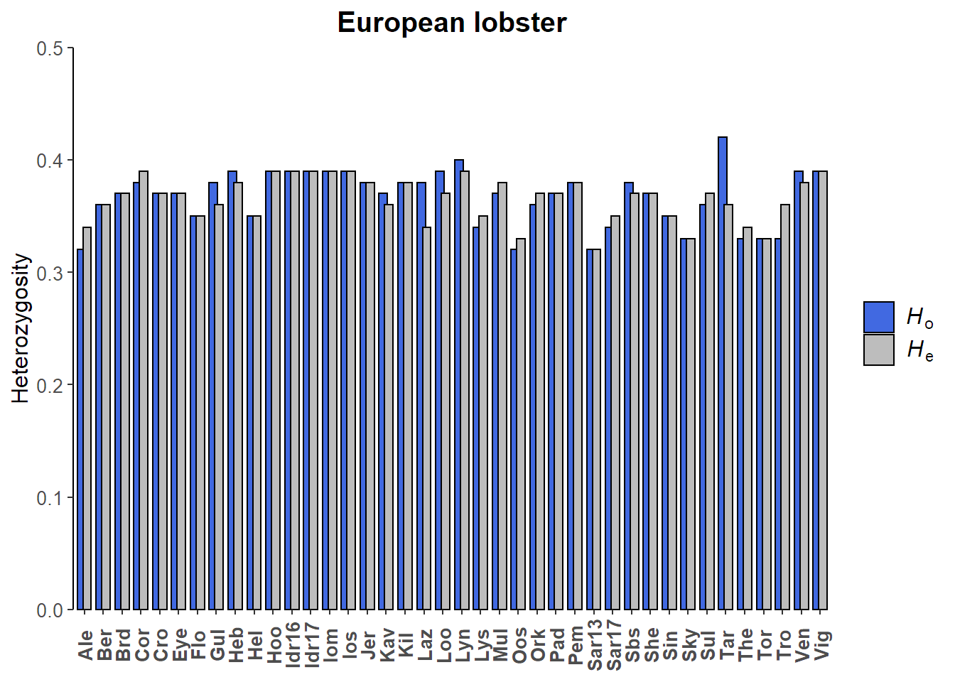
# Pink sea fan heterozygosity barplot
ggplot(data = Het_seafan_df, aes(x = Site, y = value, fill = variable))+
  geom_bar(stat = "identity", position = "dodge", colour = "black")+
  scale_y_continuous(expand = c(0,0), limits = c(0,0.60), breaks = c(0, 0.10, 0.20, 0.30, 0.40, 0.50, 0.60))+
  scale_fill_manual(values = c("pink", "#bdbdbd"), labels = c(hetlab.o, hetlab.e))+
  ylab("Heterozygosity")+
  ggtitle("Pink sea fan")+
  custom_theme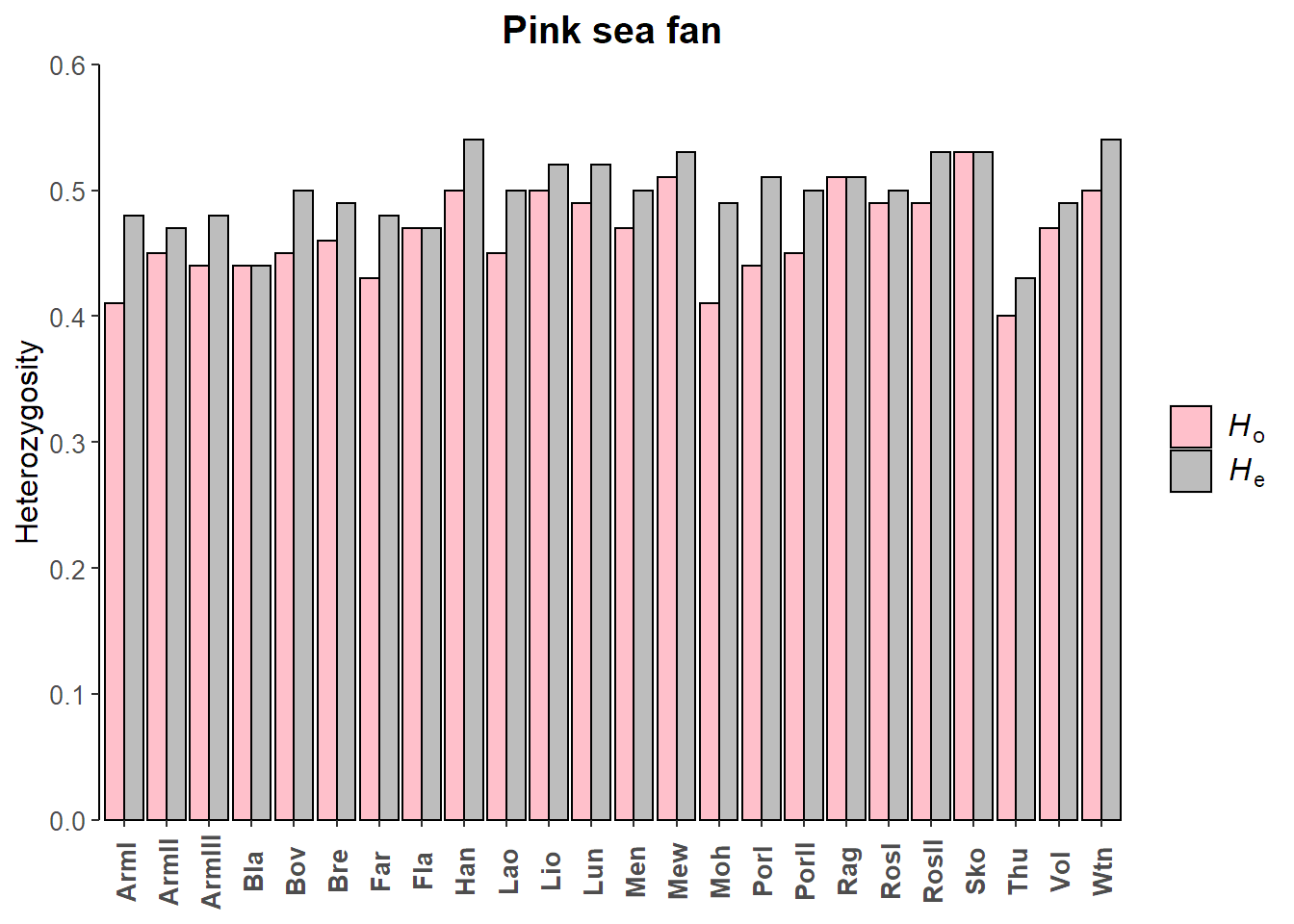
Inbreeding coefficient (FIS)
Calculate mean FIS per site.
# European lobster
apply(basic_lobster$Fis, MARGIN = 2, FUN = mean, na.rm = TRUE) %>%
  round(digits = 3)
##    Ale    Ber    Brd    Cor    Cro    Eye    Flo    Gul    Heb    Hel    Hoo
##  0.057  0.003  0.003  0.021 -0.006 -0.004  0.005 -0.044 -0.034  0.013 -0.016
##  Idr16  Idr17    Iom    Ios    Jer    Kav    Kil    Laz    Loo    Lyn    Lys
## -0.007 -0.001 -0.024 -0.007  0.004 -0.024 -0.016 -0.115 -0.043 -0.032  0.018
##    Mul    Oos    Ork    Pad    Pem  Sar13  Sar17    Sbs    She    Sin    Sky
##  0.040  0.023  0.017 -0.010 -0.004 -0.009  0.018 -0.017 -0.006 -0.013  0.006
##    Sul    Tar    The    Tor    Tro    Ven    Vig
##  0.033 -0.153  0.029  0.010  0.066 -0.024  0.013

# Pink sea fan
apply(basic_seafan$Fis, MARGIN = 2, FUN = mean, na.rm = TRUE) %>%
  round(digits = 3)
##   ArmI  ArmII ArmIII    Bla    Bov    Bre    Far    Fla    Han    Lao    Lio
##  0.166  0.085  0.076 -0.006  0.075  0.039  0.116  0.014  0.042  0.064  0.029
##    Lun    Men    Mew    Moh   PorI  PorII    Rag   RosI  RosII    Sko    Thu
##  0.057  0.067  0.030  0.153  0.137  0.089  0.010  0.048  0.077  0.013  0.056
##    Vol    Wtn
## 0.057 0.0585. FST, PCA & DAPC
FST
Compute pairwise FST (Weir & Cockerham 1984).
# Subset data sets to reduce computation time
lobster_gen_sub = popsub(lobster_gen, sublist = c("Ale","Ber","Brd","Pad","Sar17","Vig"))
seafan_gen_sub = popsub(seafan_gen, sublist = c("Bla","Bov","Bre","Lun","PorI","Sko"))
# Compute pairwise Fsts
lobster_fst = genet.dist(lobster_gen_sub, method = "WC84") %>% round(digits = 3)
lobster_fst
## Ale Ber Brd Pad Sar17
## Ber 0.120
## Brd 0.131 0.007
## Pad 0.140 0.025 0.008
## Sar17 0.066 0.174 0.171 0.161
## Vig 0.117 0.064 0.038 0.018 0.112
seafan_fst = genet.dist(seafan_gen_sub, method = "WC84") %>% round(digits = 3)
seafan_fst
## Bla Bov Bre Lun PorI
## Bov 0.099
## Bre 0.105 0.005
## Lun 0.095 -0.002 0.012
## PorI 0.114 0.052 0.045 0.045
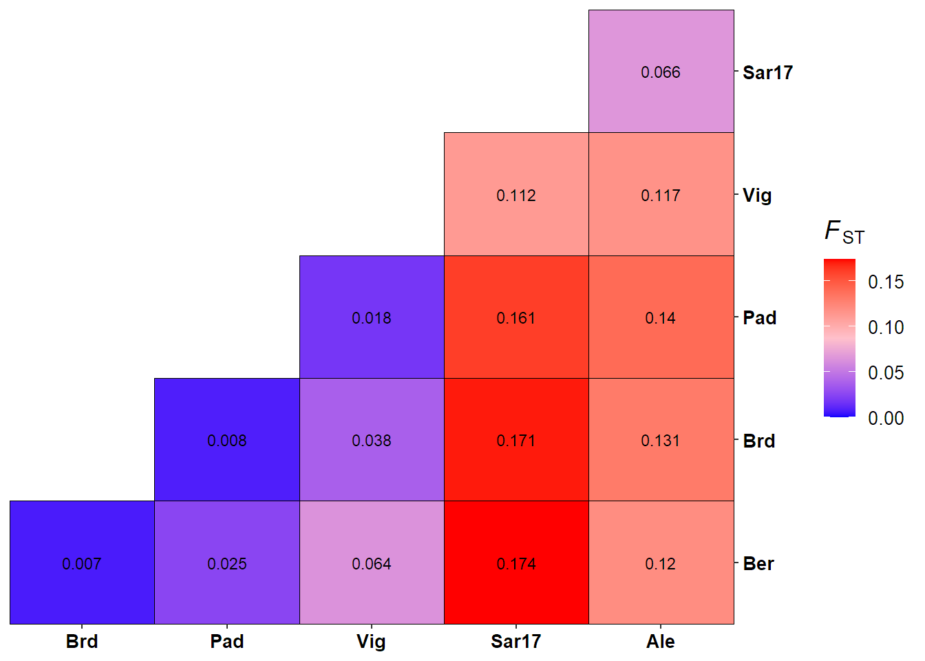
## Sko 0.094 -0.002 0.006 -0.001 0.041Visualise pairwise FST for lobster.
# Desired order of labels
lab_order = c("Ber","Brd","Pad","Vig","Sar17","Ale")

# Change order of rows and cols
fst.mat = as.matrix(lobster_fst)
fst.mat1 = fst.mat[lab_order, ]
fst.mat2 = fst.mat1[, lab_order]

# Create a data.frame
ind = which(upper.tri(fst.mat2), arr.ind = TRUE)
fst.df = data.frame(Site1 = dimnames(fst.mat2)[[2]][ind[,2]],
                    Site2 = dimnames(fst.mat2)[[1]][ind[,1]],
                    Fst = fst.mat2[ ind ])

# Keep the order of the levels in the data.frame for plotting
fst.df$Site1 = factor(fst.df$Site1, levels = unique(fst.df$Site1))
fst.df$Site2 = factor(fst.df$Site2, levels = unique(fst.df$Site2))

# Convert minus values to zero
fst.df$Fst[fst.df$Fst < 0] = 0

# Print data.frame summary
fst.df %>% str
## 'data.frame':    15 obs. of  3 variables:
##  $ Site1: Factor w/ 5 levels "Brd","Pad","Vig",..: 1 2 2 3 3 3 4 4 4 4 ...
##  $ Site2: Factor w/ 5 levels "Ber","Brd","Pad",..: 1 1 2 1 2 3 1 2 3 4 ...
##  $ Fst  : num  0.007 0.025 0.008 0.064 0.038 0.018 0.174 0.171 0.161 0.112 ...

# Fst italic label
fst.label = expression(italic("F")[ST])

# Extract middle Fst value for gradient argument
mid = max(fst.df$Fst) / 2

# Plot heatmap
ggplot(data = fst.df, aes(x = Site1, y = Site2, fill = Fst))+
  geom_tile(colour = "black")+
  geom_text(aes(label = Fst), color="black", size = 3)+
  scale_fill_gradient2(low = "blue", mid = "pink", high = "red", midpoint = mid, name = fst.label, limits = c(0, max(fst.df$Fst)), breaks = c(0, 0.05, 0.10, 0.15))+
  scale_x_discrete(expand = c(0,0))+
  scale_y_discrete(expand = c(0,0), position = "right")+
  theme(axis.text = element_text(colour = "black", size = 10, face = "bold"),
        axis.title = element_blank(),
        panel.grid = element_blank(),
        panel.background = element_blank(),
        legend.position = "right",
        legend.title = element_text(size = 14, face = "bold"),
        legend.text = element_text(size = 10)
        )
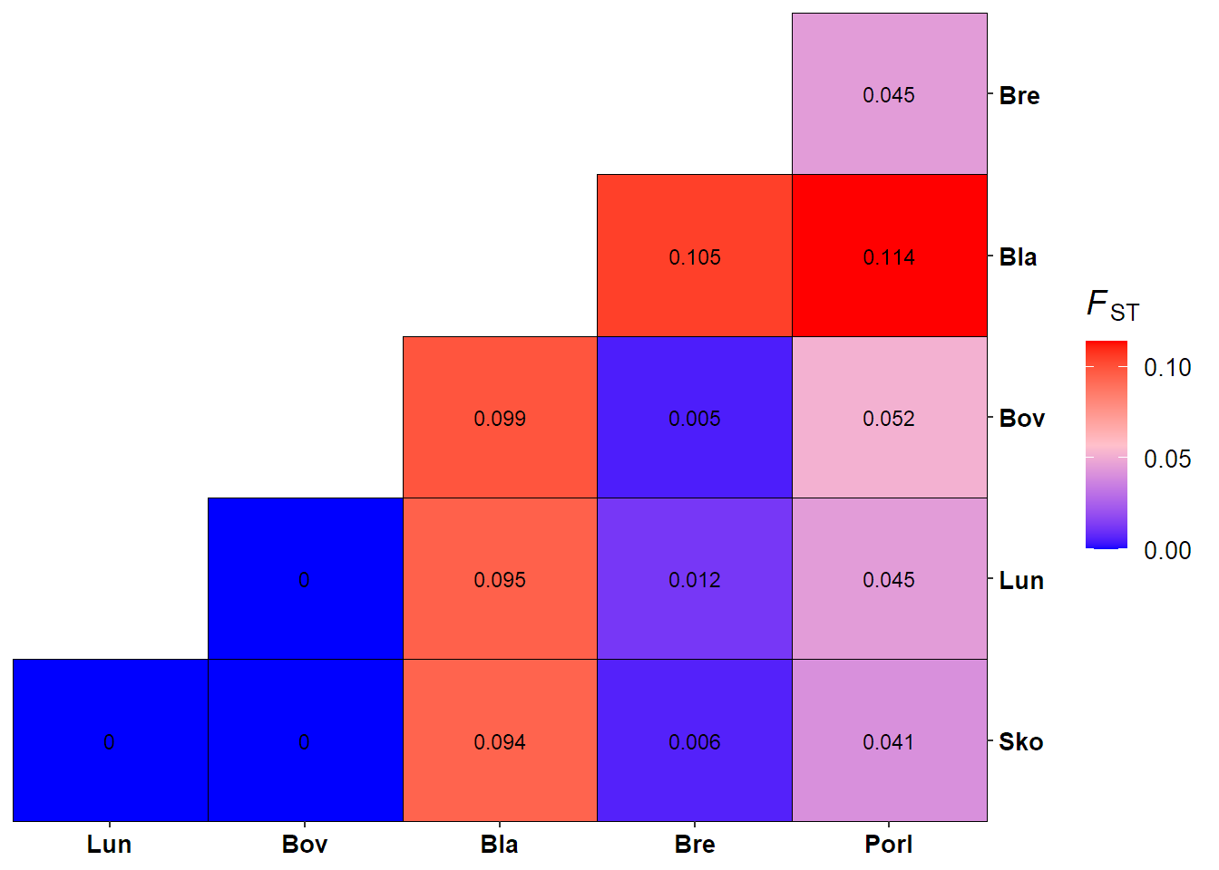
Visualise pairwise FST for pink sea fan.
# Desired order of labels
lab_order = c("Sko","Lun","Bov","Bla","Bre","PorI")

# Change order of rows and cols
fst.mat = as.matrix(seafan_fst)
fst.mat1 = fst.mat[lab_order, ]
fst.mat2 = fst.mat1[, lab_order]

# Create a data.frame
ind = which(upper.tri(fst.mat2), arr.ind = TRUE)
fst.df = data.frame(Site1 = dimnames(fst.mat2)[[2]][ind[,2]],
                    Site2 = dimnames(fst.mat2)[[1]][ind[,1]],
                    Fst = fst.mat2[ ind ])

# Keep the order of the levels in the data.frame for plotting
fst.df$Site1 = factor(fst.df$Site1, levels = unique(fst.df$Site1))
fst.df$Site2 = factor(fst.df$Site2, levels = unique(fst.df$Site2))

# Convert minus values to zero
fst.df$Fst[fst.df$Fst < 0] = 0

# Print data.frame summary
fst.df %>% str
## 'data.frame':    15 obs. of  3 variables:
##  $ Site1: Factor w/ 5 levels "Lun","Bov","Bla",..: 1 2 2 3 3 3 4 4 4 4 ...
##  $ Site2: Factor w/ 5 levels "Sko","Lun","Bov",..: 1 1 2 1 2 3 1 2 3 4 ...
##  $ Fst  : num  0 0 0 0.094 0.095 0.099 0.006 0.012 0.005 0.105 ...

# Fst italic label
fst.label = expression(italic("F")[ST])

# Extract middle Fst value for gradient argument
mid = max(fst.df$Fst) / 2

# Plot heatmap
ggplot(data = fst.df, aes(x = Site1, y = Site2, fill = Fst))+
  geom_tile(colour = "black")+
  geom_text(aes(label = Fst), color="black", size = 3)+
  scale_fill_gradient2(low = "blue", mid = "pink", high = "red", midpoint = mid, name = fst.label, limits = c(0, max(fst.df$Fst)), breaks = c(0, 0.05, 0.10))+
  scale_x_discrete(expand = c(0,0))+
  scale_y_discrete(expand = c(0,0), position = "right")+
  theme(axis.text = element_text(colour = "black", size = 10, face = "bold"),
        axis.title = element_blank(),
        panel.grid = element_blank(),
        panel.background = element_blank(),
        legend.position = "right",
        legend.title = element_text(size = 14, face = "bold"),
        legend.text = element_text(size = 10)
        )
PCA
Perform a PCA (principle components analysis) on the lobster data set.
# Replace missing data with the mean allele frequencies
x = tab(lobster_gen_sub, NA.method = "mean")

# Perform PCA
pca1 = dudi.pca(x, scannf = FALSE, scale = FALSE, nf = 3)

# Analyse how much percent of genetic variance is explained by each axis
percent = pca1$eig/sum(pca1$eig)*100
barplot(percent, ylab = "Genetic variance explained by eigenvectors (%)", ylim = c(0,12),
        names.arg = round(percent, 1))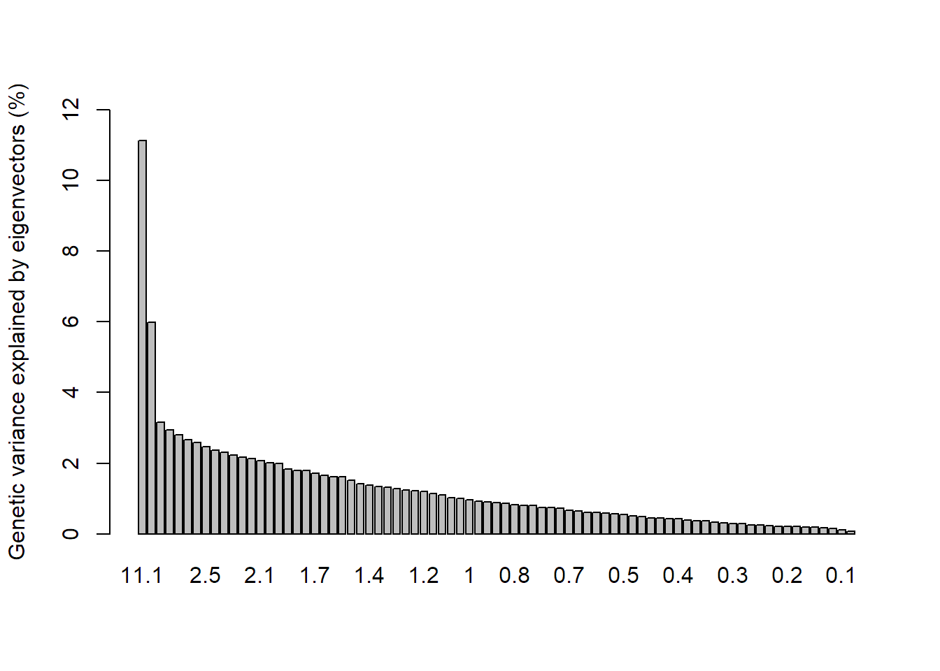
Visualise PCA results.
# Create a data.frame containing individual coordinates
ind_coords = as.data.frame(pca1$li)

# Rename columns of dataframe
colnames(ind_coords) = c("Axis1","Axis2","Axis3")

# Add a column containing individuals
ind_coords$Ind = indNames(lobster_gen_sub)

# Add a column with the site IDs
ind_coords$Site = lobster_gen_sub$pop

# Calculate centroid (average) position for each population
centroid = aggregate(cbind(Axis1, Axis2, Axis3) ~ Site, data = ind_coords, FUN = mean)

# Add centroid coordinates to ind_coords dataframe
ind_coords = left_join(ind_coords, centroid, by = "Site", suffix = c("",".cen"))

# Define colour palette
cols = brewer.pal(nPop(lobster_gen_sub), "Set1")

# Custom x and y labels
xlab = paste("Axis 1 (", format(round(percent[1], 1), nsmall=1)," %)", sep="")
ylab = paste("Axis 2 (", format(round(percent[2], 1), nsmall=1)," %)", sep="")

# Custom theme for ggplot2
ggtheme = theme(axis.text.y = element_text(colour="black", size=12),
                axis.text.x = element_text(colour="black", size=12),
                axis.title = element_text(colour="black", size=12),
                panel.border = element_rect(colour="black", fill=NA, size=1),
                panel.background = element_blank(),
                plot.title = element_text(hjust=0.5, size=15)
)

# Scatter plot axis 1 vs. 2
ggplot(data = ind_coords, aes(x = Axis1, y = Axis2))+
  geom_hline(yintercept = 0)+
  geom_vline(xintercept = 0)+
  # spider segments
  geom_segment(aes(xend = Axis1.cen, yend = Axis2.cen, colour = Site), show.legend = FALSE)+
  # points
  geom_point(aes(fill = Site), shape = 21, size = 3, show.legend = FALSE)+
  # centroids
  geom_label(data = centroid, aes(label = Site, fill = Site), size = 4, show.legend = FALSE)+
  # colouring
  scale_fill_manual(values = cols)+
  scale_colour_manual(values = cols)+
  # custom labels
  labs(x = xlab, y = ylab)+
  ggtitle("Lobster PCA")+
  # custom theme
  ggtheme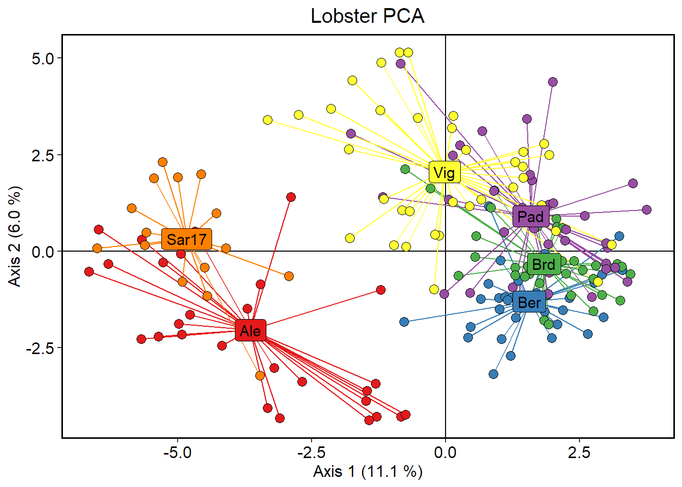
# Export plot
# ggsave("Figure1.png", width = 12, height = 8, dpi = 600)
DAPC
Perform a DAPC (discriminant analysis of principal components) on the seafan data set.
# Perform cross validation to find the optimal number of PCs to retain in DAPC
set.seed(123)
x = tab(seafan_gen_sub, NA.method = "mean")
crossval = xvalDapc(x, seafan_gen_sub$pop, result = "groupMean", xval.plot = TRUE)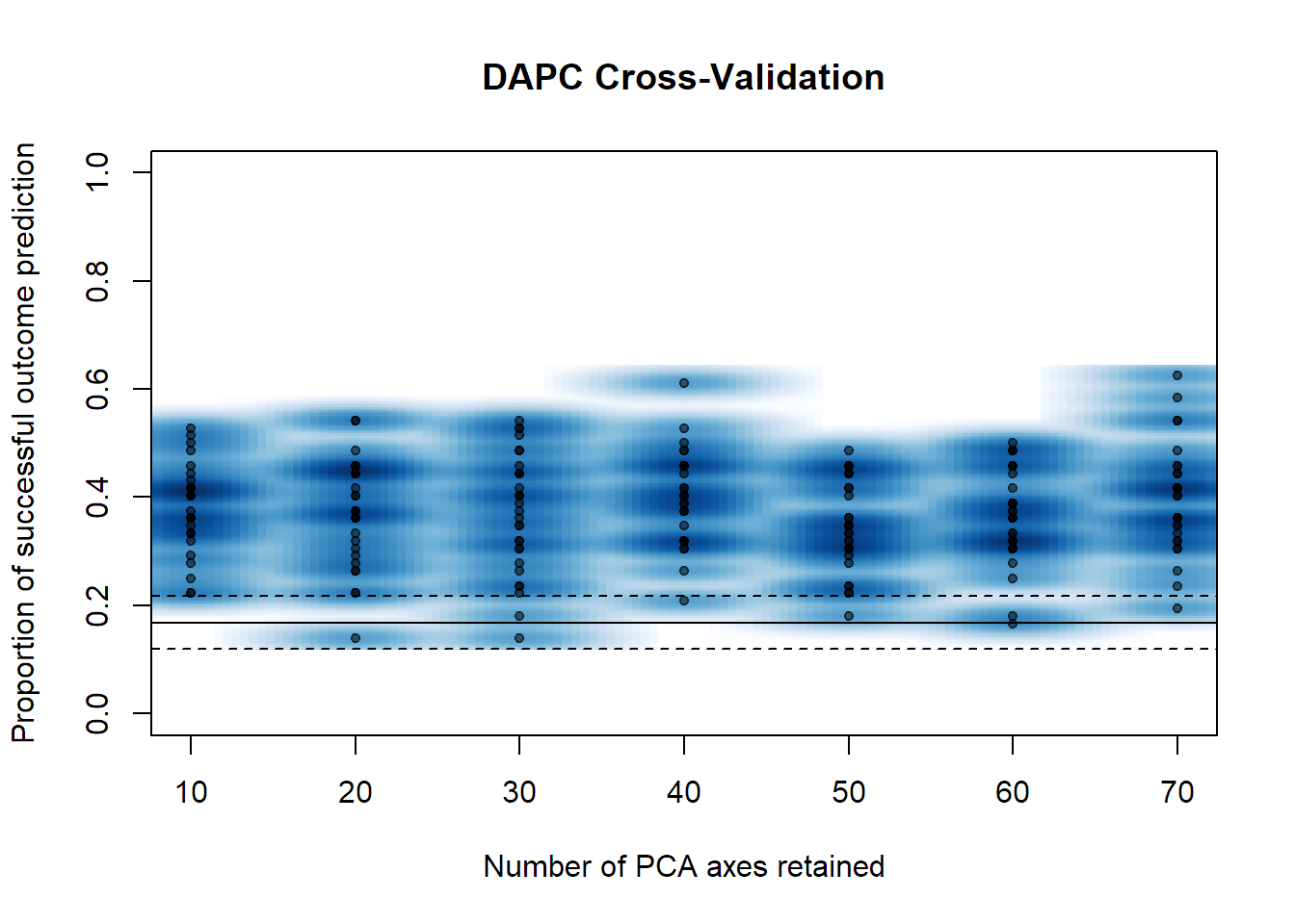
# Number of PCs with best stats (lower score = better)
crossval$`Root Mean Squared Error by Number of PCs of PCA`
##        10        20        30        40        50        60        70
## 0.6252777 0.6326131 0.6380681 0.6057849 0.6587395 0.6412447 0.6113320
crossval$`Number of PCs Achieving Highest Mean Success`
## [1] "40"
crossval$`Number of PCs Achieving Lowest MSE`
## [1] "40"
numPCs = as.numeric(crossval$`Number of PCs Achieving Lowest MSE`)
# Run a DAPC using site IDs as priors
dapc1 = dapc(seafan_gen_sub, seafan_gen_sub$pop, n.pca = numPCs, n.da = 3)
# Analyse how much percent of genetic variance is explained by each axis
percent = dapc1$eig/sum(dapc1$eig)*100
barplot(percent, ylab = "Genetic variance explained by eigenvectors (%)", ylim = c(0,60),
names.arg = round(percent, 1))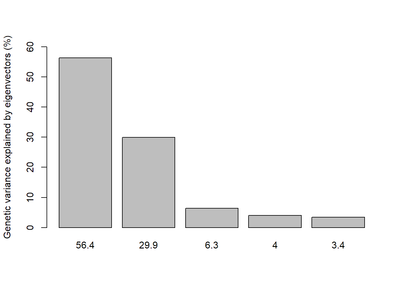
Visualise DAPC results.
# Create a data.frame containing individual coordinates
ind_coords = as.data.frame(dapc1$ind.coord)

# Rename columns of dataframe
colnames(ind_coords) = c("Axis1","Axis2","Axis3")

# Add a column containing individuals
ind_coords$Ind = indNames(seafan_gen_sub)

# Add a column with the site IDs
ind_coords$Site = seafan_gen_sub$pop

# Calculate centroid (average) position for each population
centroid = aggregate(cbind(Axis1, Axis2, Axis3) ~ Site, data = ind_coords, FUN = mean)

# Add centroid coordinates to ind_coords dataframe
ind_coords = left_join(ind_coords, centroid, by = "Site", suffix = c("",".cen"))

# Define colour palette
cols = brewer.pal(nPop(seafan_gen_sub), "Set2")

# Custom x and y labels
xlab = paste("Axis 1 (", format(round(percent[1], 1), nsmall=1)," %)", sep="")
ylab = paste("Axis 2 (", format(round(percent[2], 1), nsmall=1)," %)", sep="")

# Scatter plot axis 1 vs. 2
ggplot(data = ind_coords, aes(x = Axis1, y = Axis2))+
  geom_hline(yintercept = 0)+
  geom_vline(xintercept = 0)+
  # spider segments
  geom_segment(aes(xend = Axis1.cen, yend = Axis2.cen, colour = Site), show.legend = FALSE)+
  # points
  geom_point(aes(fill = Site), shape = 21, size = 3, show.legend = FALSE)+
  # centroids
  geom_label(data = centroid, aes(label = Site, fill = Site), size = 4, show.legend = FALSE)+
  # colouring
  scale_fill_manual(values = cols)+
  scale_colour_manual(values = cols)+
  # custom labels
  labs(x = xlab, y = ylab)+
  ggtitle("Pink sea fan DAPC")+
  # custom theme
  ggtheme
# Export plot
# ggsave("Figure2.png", width = 12, height = 8, dpi = 600)6. Extras
Import VCF file
To illustrate importing VCF files and conducting OutFLANK outlier selection tests in R, we will use an American lobster SNP data set available from the Dryad Digital Repository.
# Load vcfR package
library(vcfR)

# Import only 3,000 variants to reduce computation time
american = read.vcfR("10156-586.recode.vcf", nrows = 3000, verbose = FALSE)
american
## ***** Object of Class vcfR *****
## 586 samples
## 1 CHROMs
## 3,000 variants
## Object size: 16.6 Mb
## 0 percent missing data
## *****        *****         *****

# Convert to genind object
american = vcfR2genind(american)

# Add site IDs to genind object
american$pop = as.factor(substr(indNames(american), 1, 3))Conduct outlier tests using OutFLANK
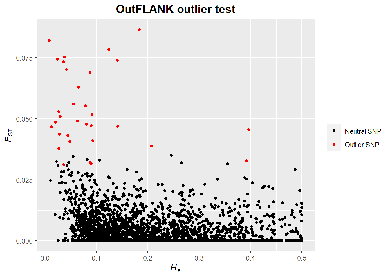
Conduct FST differentiation-based outlier tests on genind object using OutFLANK using a wrapper script from the dartR package.
# Load packages
library(OutFLANK)
library(qvalue)
library(dartR)
# Run OutFLANK using dartR wrapper script
outflnk = gl.outflank(american, qthreshold = 0.05, plot = FALSE)
## Calculating FSTs, may take a few minutes...
# Extract OutFLANK results
outflnk.df = outflnk$outflank$results
# Remove duplicated rows for each SNP locus
rowsToRemove = seq(1, nrow(outflnk.df), by = 2)
outflnk.df = outflnk.df[-rowsToRemove, ]
# Print number of outliers (TRUE)
outflnk.df$OutlierFlag %>% summary
## Mode FALSE TRUE
## logical 2968 32# Extract outlier IDs
outlier_indexes = which(outflnk.df$OutlierFlag == TRUE)
outlierID = locNames(american)[outlier_indexes]
outlierID
## [1] "un-11566" "un-69080" "un-111790" "un-111865" "un-125908" "un-172034"
## [7] "un-186923" "un-201848" "un-205435" "un-243757" "un-253632" "un-257077"
## [13] "un-288280" "un-288327" "un-342055" "un-395275" "un-395276" "un-424882"
## [19] "un-433799" "un-493905" "un-525474" "un-531991" "un-541424" "un-561940"
## [25] "un-581802" "un-631261" "un-631875" "un-649002" "un-676856" "un-679035"
## [31] "un-691876" "un-734068"# Convert Fsts <0 to zero
outflnk.df$FST[outflnk.df$FST < 0] = 0
# Italic labels
fstlab = expression(italic("F")[ST])
hetlab = expression(italic("H")[e])
# Plot He versus Fst
ggplot(data = outflnk.df)+
geom_point(aes(x = He, y = FST, colour = OutlierFlag))+
scale_colour_manual(values = c("black","red"), labels = c("Neutral SNP","Outlier SNP"))+
ggtitle("OutFLANK outlier test")+
xlab(hetlab)+
ylab(fstlab)+
theme(legend.title = element_blank(),
plot.title = element_text(hjust = 0.5, size = 15, face = "bold")
)
Export biallelic SNP genind object
Load required packages.
library(devtools)
library(miscTools)
library(stringr)
Export genind object in genepop format.
source_url("https://raw.githubusercontent.com/Tom-Jenkins/utility_scripts/master/TJ_genind2genepop_function.R")
genind2genepop(lobster_gen_sub, file = "lobster_genotypes.gen")
Export genind object in STRUCTURE format. If you want to run STRUCTURE in Linux then use unix = TRUE which exports a Unix text file (Windows text file by default).
source_url("https://raw.githubusercontent.com/Tom-Jenkins/utility_scripts/master/TJ_genind2structure_function.R")
genind2structure(lobster_gen_sub, file = "lobster_genotypes.str", pops = TRUE, markers = TRUE, unix = FALSE)Further resources
Conduct and visualise admixture analyses in R
Population genetics and genomics in R
Detecting multilocus adaptation using redundancy analysis
Using pcadapt to detect local adaptation
Analysis of multilocus genotypes and lineages in poppr
Spatial analysis of principal components analysis using adegenet
Download a PDF of this post
R session info
sessionInfo()
## R version 4.1.2 (2021-11-01)
## Platform: x86_64-w64-mingw32/x64 (64-bit)
## Running under: Windows 10 x64 (build 19043)
##
## Matrix products: default
##
## locale:
## [1] LC_COLLATE=English_United Kingdom.1252
## [2] LC_CTYPE=English_United Kingdom.1252
## [3] LC_MONETARY=English_United Kingdom.1252
## [4] LC_NUMERIC=C
## [5] LC_TIME=English_United Kingdom.1252
##
## attached base packages:
## [1] stats     graphics  grDevices utils     datasets  methods   base
##
## other attached packages:
##  [1] stringr_1.4.0      miscTools_0.6-26   devtools_2.4.3     usethis_2.1.5
##  [5] dartR_2.0.3        OutFLANK_0.2       qvalue_2.26.0      vcfR_1.12.0
##  [9] scales_1.1.1       RColorBrewer_1.1-2 ggplot2_3.3.5      reshape2_1.4.4
## [13] hierfstat_0.5-10   dplyr_1.0.8        poppr_2.9.3        adegenet_2.1.5
## [17] ade4_1.7-18
##
## loaded via a namespace (and not attached):
##   [1] spam_2.8-0          StAMPP_1.6.3        plyr_1.8.6
##   [4] igraph_1.3.0        sp_1.4-6            splines_4.1.2
##   [7] digest_0.6.29       foreach_1.5.2       htmltools_0.5.2
##  [10] viridis_0.6.2       gdata_2.18.0        fansi_1.0.2
##  [13] magrittr_2.0.2      memoise_2.0.1       cluster_2.1.2
##  [16] doParallel_1.0.17   PopGenReport_3.0.4  remotes_2.4.2
##  [19] R.utils_2.11.0      prettyunits_1.1.1   colorspace_2.0-2
##  [22] mmod_1.3.3          xfun_0.29           rgdal_1.5-29
##  [25] callr_3.7.0         crayon_1.5.0        jsonlite_1.7.3
##  [28] iterators_1.0.14    ape_5.6-1           glue_1.6.1
##  [31] gtable_0.3.0        seqinr_4.2-8        polysat_1.7-6
##  [34] pkgbuild_1.3.1      maps_3.4.0          mvtnorm_1.1-3
##  [37] DBI_1.1.2           GGally_2.1.2        Rcpp_1.0.8
##  [40] viridisLite_0.4.0   xtable_1.8-4        dotCall64_1.0-1
##  [43] dismo_1.3-5         genetics_1.3.8.1.3  calibrate_1.7.7
##  [46] ellipsis_0.3.2      pkgconfig_2.0.3     reshape_0.8.8
##  [49] R.methodsS3_1.8.1   farver_2.1.0        sass_0.4.0
##  [52] utf8_1.2.2          tidyselect_1.1.1    labeling_0.4.2
##  [55] rlang_1.0.1         later_1.3.0         munsell_0.5.0
##  [58] tools_4.1.2         cachem_1.0.6        cli_3.1.1
##  [61] generics_0.1.2      evaluate_0.14       fastmap_1.1.0
##  [64] yaml_2.2.2          processx_3.5.2      knitr_1.37
##  [67] fs_1.5.2            gdsfmt_1.30.0       purrr_0.3.4
##  [70] RgoogleMaps_1.4.5.3 nlme_3.1-153        mime_0.12
##  [73] R.oo_1.24.0         brio_1.1.3          gap_1.2.3-1
##  [76] compiler_4.1.2      rstudioapi_0.13     png_0.1-7
##  [79] testthat_3.1.2      tibble_3.1.6        bslib_0.3.1
##  [82] stringi_1.7.6       ps_1.6.0            gdistance_1.3-6
##  [85] highr_0.9           blogdown_1.9        desc_1.4.0
##  [88] fields_13.3         memuse_4.2-1        lattice_0.20-45
##  [91] Matrix_1.3-4        vegan_2.5-7         permute_0.9-7
##  [94] vctrs_0.3.8         pillar_1.7.0        lifecycle_1.0.1
##  [97] combinat_0.0-8      jquerylib_0.1.4     data.table_1.14.2
## [100] SNPRelate_1.28.0    raster_3.5-15       httpuv_1.6.5
## [103] patchwork_1.1.1     R6_2.5.1            bookdown_0.25
## [106] promises_1.2.0.1    KernSmooth_2.23-20  gridExtra_2.3
## [109] sessioninfo_1.2.2   codetools_0.2-18    pkgload_1.2.4
## [112] boot_1.3-28         MASS_7.3-54         gtools_3.9.2
## [115] assertthat_0.2.1    rprojroot_2.0.2     withr_2.4.3
## [118] pinfsc50_1.2.0      pegas_1.1           mgcv_1.8-38
## [121] parallel_4.1.2      terra_1.5-21        grid_4.1.2
## [124] tidyr_1.2.0         rmarkdown_2.13      shiny_1.7.1